17 Models
Summary
A model is a simplification of the real world that helps us make decisions and predictions.
The variables used to make predictions are called prediction variables, while the variables we are trying to predict are called response variables.
If these are numerical, the difference between a prediction and the response is called the error or residual.
optim This is a general purpose optimization function that maximizes or minimizes a function. It is part of the stats package that is always loaded into R.
17.1 Modeling data
Once data has been cleaned and tidied, and some visualizations have been created in order to see what is going on, often a pattern emerges. What is the next step? A key piece of data science methodology is modeling your data, in order to create predictions. A model is a simplification of the real world that allows us to predict outcomes.
For instance, a map is a model that is very useful.
Figure 17.1: A map of the Claremont Colleges
A map does not try to incorporate every building, every tree, or every bush in a given location. It does not record the markings on the middle of a road because they do not matter to the purpose of the map. That is because the location of the roads is useful when planning a route, while knowing the trees on the side of the road are usually not.
Instead, a model seeks to capture what is important about the thing that it is modeling. It allows the user to make informed decisions, and understand what is important in the data, and what is not.
This notion is captured by a famous paraphrase of George Box: “All models are wrong, but some are useful.” No model completely captures the nature of the thing it is modeling. A useful model strips away unnecessary information to leave you with a bare bones skeleton that tries to capture the essence of what is going on.
17.2 Linear models
The simplest relationship between two observed variables is linear. Sometimes this relationship is formed by definition. Since an inch is 2.54 centimeters, one’s height in inches varies linearly with one’s height in centimeters.
Other times the connection is more tenuous: does one’s performance on a test vary linearly with the amount of time one studies? This simple model can be written as \[ y = c_0 + c_1 x. \] Here there are two parameters in the model, \(c_0\) and \(c_1\). Of course, such a line never fits real data precisely, so instead the model could be \[ y_i = c_0 + c_1 x_i + \epsilon_i, \] where \((x_i,y_i)\) is the \(i\)th observation, and \(\epsilon_i\) is what is called an error or random effect. Typically \(\epsilon_i\) is modeled as a random variable. A random variable is a variable about which we have partial information. So while a random variable is not known exactly, something about it is known. For instance, \(\epsilon_i\) can be modeled as having an equal chance of being positive or negative.
In the modelr package, there is a simulated dataset sim1 to try out these ideas. Consider this data.
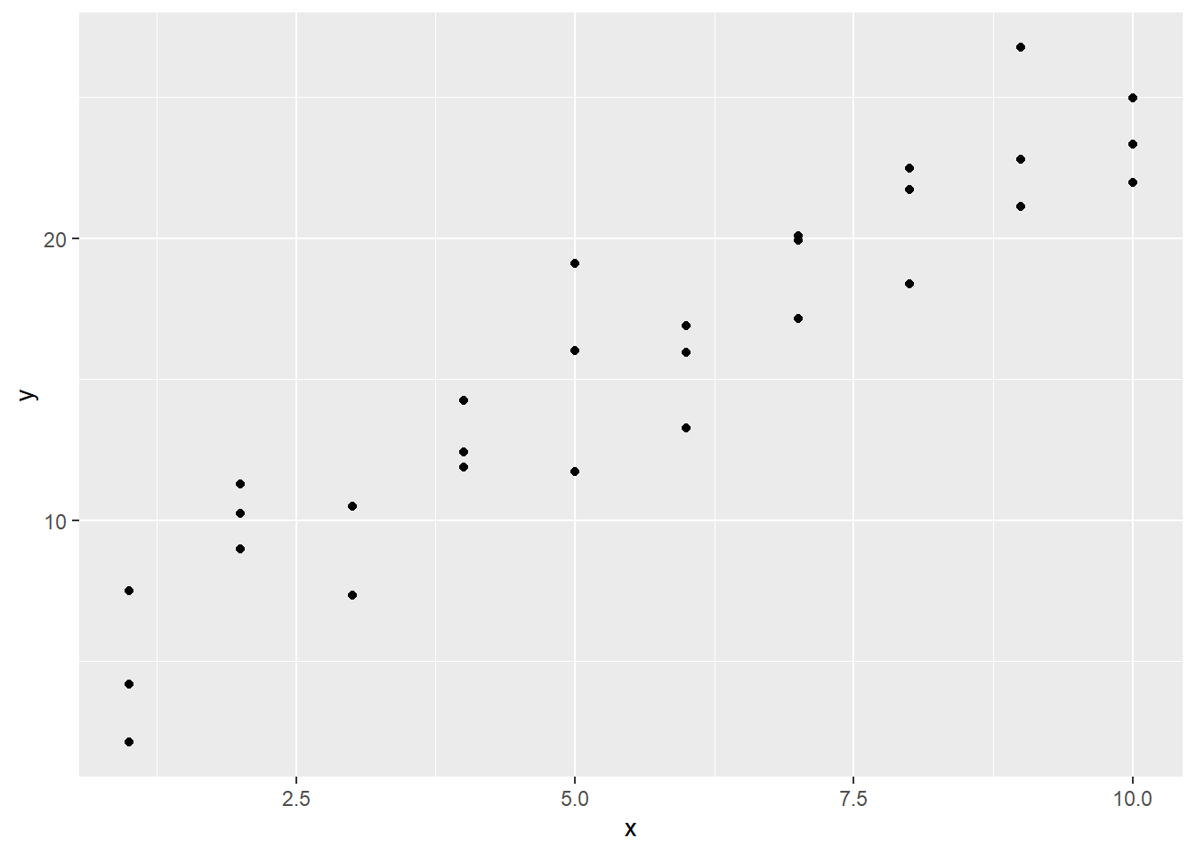
The visualization reveals that a linear model is not too far off: the \(y_i\) values look like they are varying roughly linearly on the \(x_i\) values. But here is an important note: do not get too caught up in the \(x\) versus \(y\) distinction. If the axis of \(x\) and \(y\) that vary linearly had been swapped, it also results in a linear relationship!
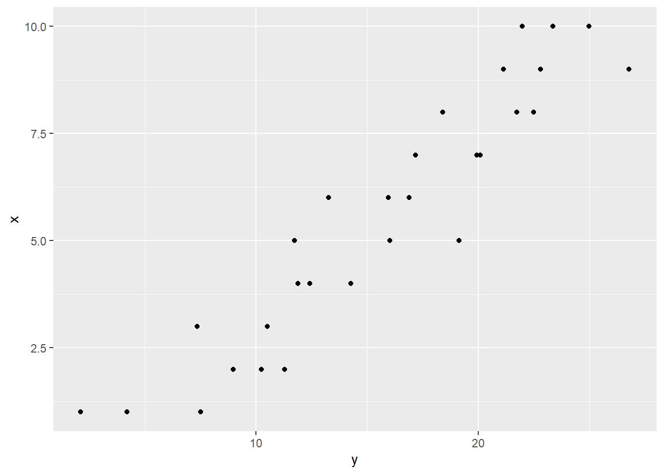
It is not the case that \(x\) causes \(y\), or the other way around. This modeling relationship is for prediction only.
With all that said, note that there does exist an asymmetry in the data: for each value \(x\) can take on, \(y\) can take on multiple values. And the values that the \(x_i\) can take on are positive integers.
## # A tibble: 30 × 2
##        x     y
##    <int> <dbl>
##  1     1  4.20
##  2     1  7.51
##  3     1  2.13
##  4     2  8.99
##  5     2 10.2
##  6     2 11.3
##  7     3  7.36
##  8     3 10.5
##  9     3 10.5
## 10     4 12.4
## # ℹ 20 more rows
Therefore, in this case it makes more sense to model \(y_i = c_0 + c_1 x_i + \epsilon_i\) than the other way around. This raises the question: what should \(c_0\) and \(c_1\) be?
A simple way of doing this would be to choose the line that passes through the middle \(y\) value when \(x = 1\), and the middle \(y\) value when \(x = 10\).
## # A tibble: 6 × 2
##       x     y
##   <int> <dbl>
## 1     1  2.13
## 2     1  4.20
## 3     1  7.51
## 4    10 22.0
## 5    10 23.3
## 6    10 25.0
So this line is \(y_i = (x - 1)(23.34 - 4.2)/(10 - 1) + 4.2 = 2.12x + 2.08.\) We can put this on the plot of the data with the geom_abline function.
sim1 |>
  ggplot(aes(x, y)) +
  geom_point() +
  geom_abline(aes(intercept = 2.08, slope = 2.12),
              col = "blue", lwd = 1)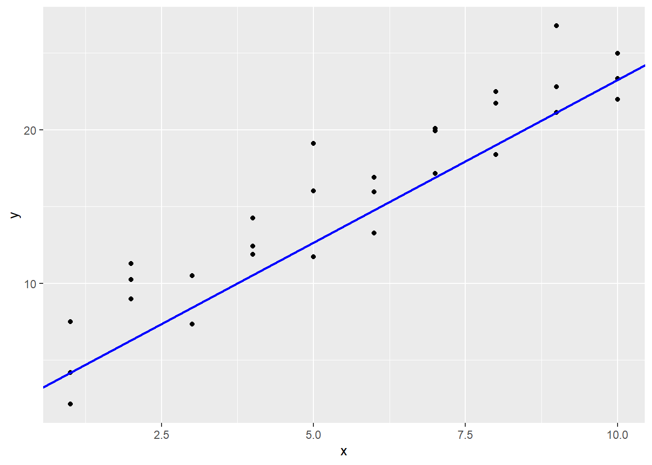
It does look okay, but maybe it is a little low for this data? One way to more objectively see how well we are doing is to measure the errors \(\epsilon_i\). The mutate function can be used in this calculation, which draws a line segment from the prediction line to the real \(y\) values.
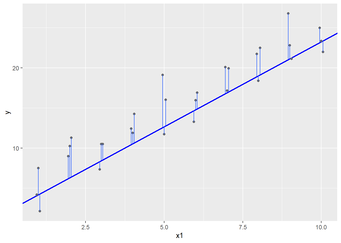
Given a model \(y_i = c_0 + c_1 x_i + \epsilon_i\) and estimates \(\hat c_0\) and \(\hat c_1\) for \(c_0\) and \(c_1\), call \(\hat y_i = \hat c_0 + \hat c_1 x_i\) the prediction, \(y_i\) the response, and \(y_i - \hat y_i\) the error or residual.
In an ideal world, all the errors would be zero and the prediction would exactly match the response. This never happens in real numerical data though: there are just too many ways for the measurement to go wrong or for the model to not exactly capture the process.
So instead just try to make the magnitude of the error as small as possible. Without going into too much detail why, the most common way of modeling the error is to use a normal random variable centered at 0. This leads to something in statistics called the maximum likelihood estimate, or MLE. For us, the important thing about the MLE is that it occurs at the place where the sum of the squares of the residuals are as small as possible.
In a model, the choice of parameters that minimizes the sum of the squares of the errors is called the least squares fit.
To find these errors, consider making a function that is our model. The function takes a tibble or data frame with variable x, and adds a prediction variable given the slope and intercept of a linear model. Once the prediction is known, the residuals can be calculated.
## # A tibble: 30 × 4
##        x     y  pred    resid
##    <int> <dbl> <dbl>    <dbl>
##  1     1  4.20  4.19  0.00991
##  2     1  7.51  4.19  3.32
##  3     1  2.13  4.19 -2.06
##  4     2  8.99  6.31  2.68
##  5     2 10.2   6.31  3.93
##  6     2 11.3   6.31  4.99
##  7     3  7.36  8.43 -1.07
##  8     3 10.5   8.43  2.08
##  9     3 10.5   8.43  2.08
## 10     4 12.4  10.6   1.88
## # ℹ 20 more rows
So now the table contains both predicted and residual values. Now measure the sum of the squares of the error, when the response values are in variable y.
sum_square_error <- function(c, data) {
  SS <-
    data |>
    mutate(pred  = c[1] + c[2] * x,
           resid = y - pred) |>
    summarize(sum(resid^2)) |>
    as.double()
  return(SS)
}
Now try this on our data:
## [1] 231.4741Now consider trying to make this sum_square_error smaller by pushing the line up a little bit.
## [1] 228.3075Better! By playing around with the intercept and slope, this squared error sum can be made much smaller. In fact, R has a built in function to do exactly that. It is called optim, and it works using a method called Newton-Raphson.
Applying this method to the sim1 data can be accomplished as follows. The first argument is a starting point for the parameters. The second is the function to be minimized. The third gives any parameters to the function beyond the original parameters.
## $par
## [1] 4.220941 2.051548
##
## $value
## [1] 135.8746
##
## $counts
## function gradient
##       65       NA
##
## $convergence
## [1] 0
##
## $message
## NULL
The output is a list of different outputs. The parameters of best fit are called par. The actual least sum of squares is given in the value piece, which is 135.8746 here, better than our earlier models.
Now assign this to a variable.
To pull the fitted parameters in par out from the list, either the $ operator can be used, or the double bracket operator can be used.
First use $par:
## [1] 4.220941 2.051548Next, use [[1]] to pull out the first piece of the variable.
## [1] 4.220941 2.051548Finally, use the double bracket with the name of the part of the variable to be extracted.
## [1] 4.220941 2.051548Whatever method is used, the result is the fitted parameters to the model that has the least squares of errors.
So our slope was pretty good to start with, but our intercept needed to be quite a bit higher. Plotting this line with optimal sum of squared error gives:
sim1 |>
  ggplot(aes(x, y)) +
  geom_point() +
  geom_abline(aes(intercept = 4.22, slope = 2.05),
              col = "blue", lwd = 1)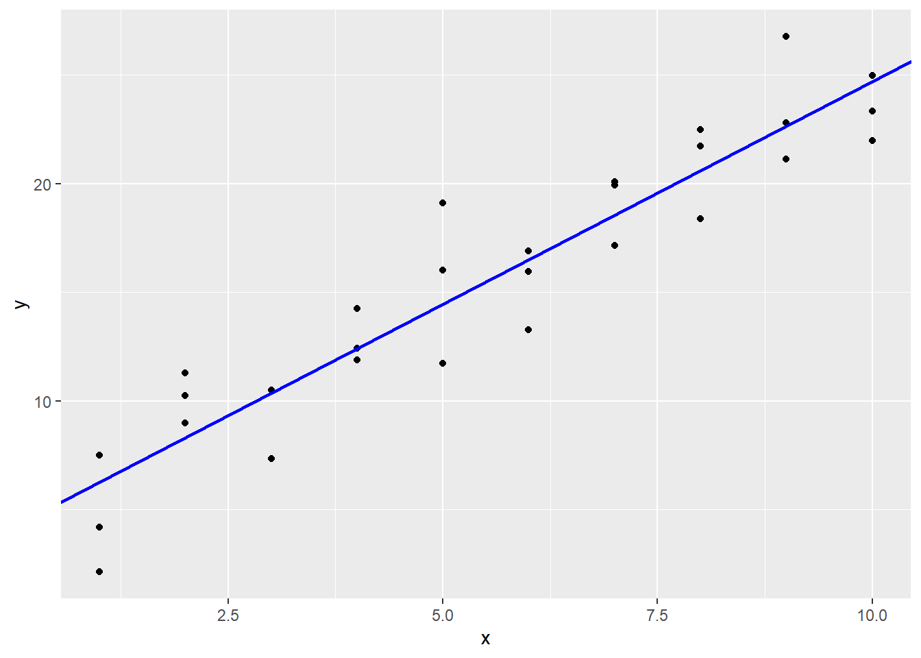
Note that in running optim, the function sum_square_error was passed as a parameter. Being able to pass functions as input to other functions is part of a way of computing called functional programming.
The square root of the sum of squares of a vector is also called the \(L_2\)-distance (or Euclidean distance). Another way of measuring the distance is the \(L_1\)-distance, which is the sum of the absolute values of the vector. With this, we get a slightly different line:
sum_abs_error <- function(c, data) {
  sum_abs <-
    data |>
    mutate(pred  = c[1] + c[2] * x,
           resid = y - pred) |>
    summarize(sum(abs(resid))) |>
    as.double()
  return(sum_abs)
}## [1] 4.364846 2.048918Go ahead and graph it.
sim1 |>
  ggplot(aes(x, y)) +
  geom_point() +
  geom_abline(aes(intercept = optimal_coef$par[1],
                  slope = optimal_coef$par[2]),
              col = "blue", lwd = 1, alpha = 0.2) +
  geom_abline(aes(intercept = optimal_coef2$par[1],
                  slope = optimal_coef2$par[2]),
              col = "red", lwd = 1, alpha = 0.2)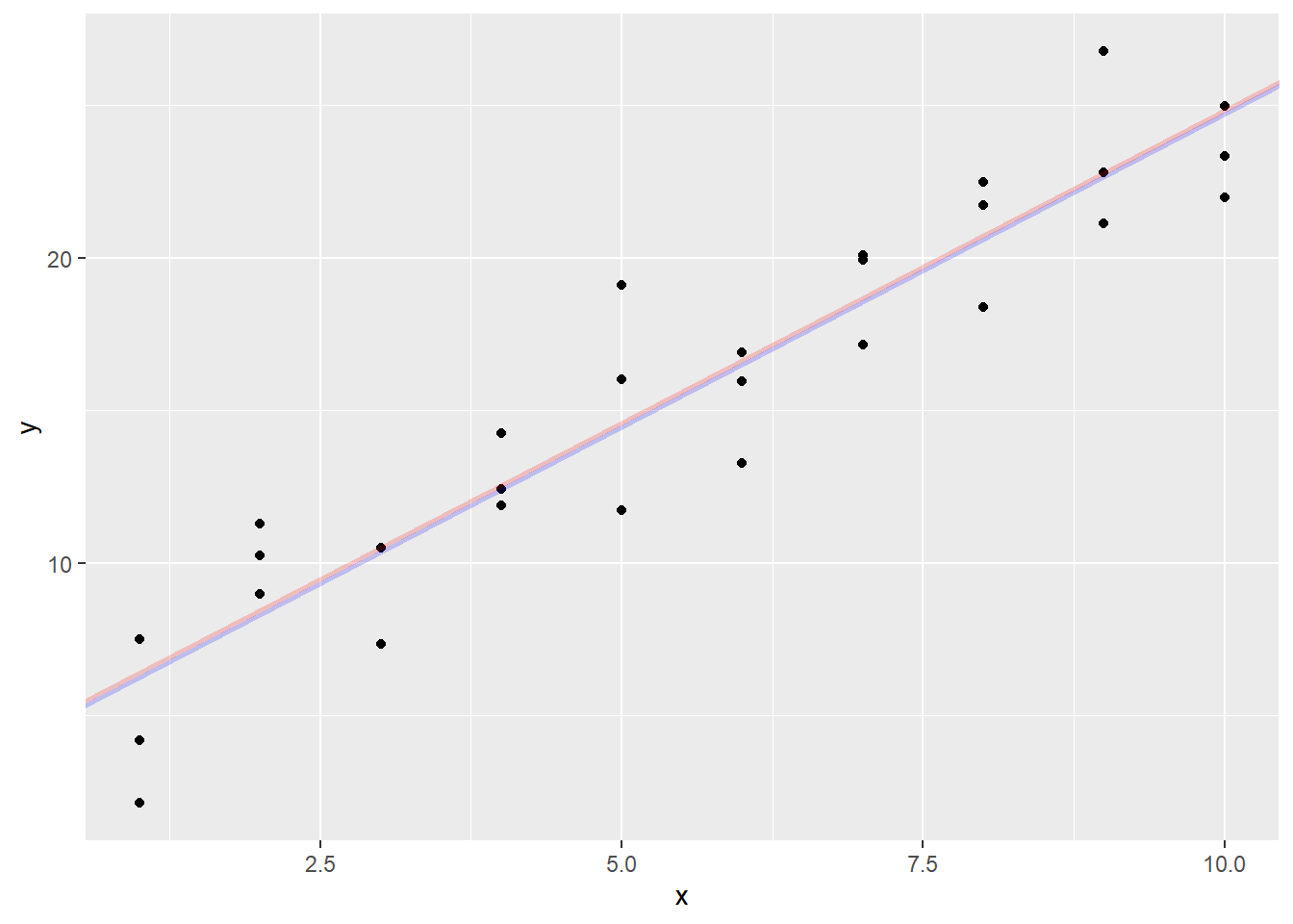
In this case, the two lines are pretty much on top of each other, but if I have an outlier, a point far away from the group, it will drag the \(L_2\)-distance (least squares) line much more than the \(L_1\)-distance line.
Let’s test that by creating a point with \(x = 10\) and \(y = 60\).
Now compute the new estimates for the coefficients
## [1] 2.113961 2.626251## [1] 4.358070 2.051177Now graph the new estimates
sim1aug |>
  ggplot(aes(x, y)) +
  geom_point() +
  geom_abline(aes(intercept = optimal_coef3$par[1],
    slope = optimal_coef3$par[2]), col = "blue",
    lwd = 1, alpha = 0.2) +
  geom_abline(aes(intercept = optimal_coef4$par[1],
    slope = optimal_coef4$par[2]), col = "red",
    lwd = 1, alpha = 0.2)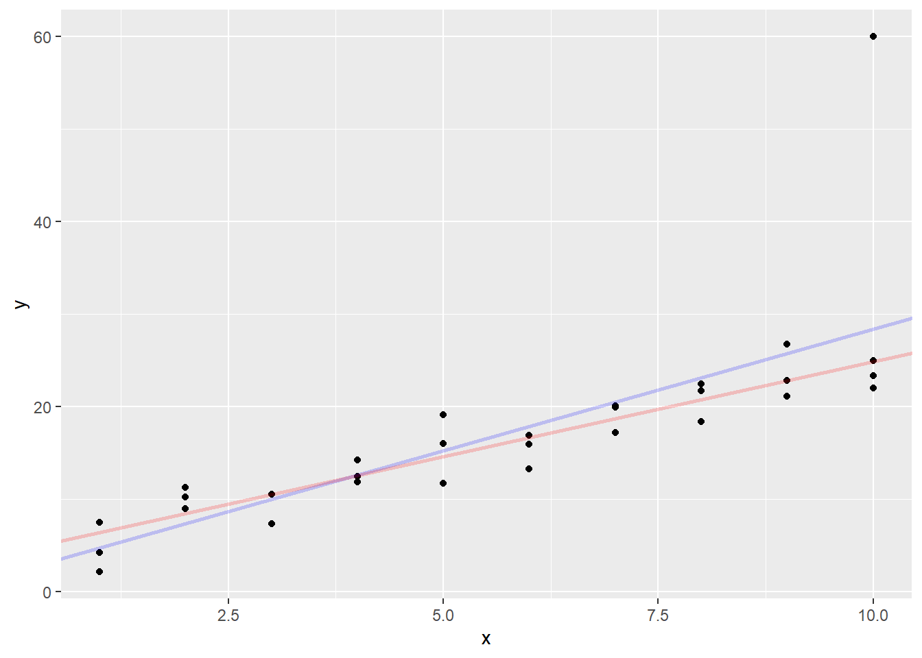
The least squares line was pulled a good distance away from the main body of the points. However, the absolute value line almost stayed in position. The outlier affected its slope much less than the least squares line.
It is important to note that neither of these lines are “right” in the sense of one being objectively better than the other, but they are both useful in making predictions. The least squares line is used most often because it is easier to calculate, but for small problems, the least absolute value line is less influenced by outliers.