15 Introduction to Structured Query Language (SQL)
Summary
First are commands to connect and disconnect from a remote database.
dbConnect
dbDisconnect.
SQL, Structured Query Language, is a way to draw out data from a centrally maintained database. It is designed to be written to make commands clear while providing much of the same power for selecting and transforming data seen earlier in the tidyverse. Because the tidyverse was written with SQL in mind, some dplyr functions have similar names.
SELECT is like select in dplyr, and will pick out a subset of variables/factors.
WHERE is like filter in dplyr, it picks out observations meeting certain criteria.
ORDER BY is like arrange in dplyr, it orders the returned observations by one or more variables.
NULL is like NA, and denotes data that is missing or unavailable.
IS NULL is like is.na, and checks to see if the variable value is NULL
AND is like &, and is used for the logical and.
OR is like |, and is used for the logical or.
NOT is like !, and is used for the logical not.
AS is like mutate in dplyr, and is used for building new variables from existing ones.
LIKE is like str_extract in stringr, and pulls out observations involving strings.
LIMIT is like head or slice, and only returns the first few values found.
OFFSET returns some observations after skipping some at the beginning.
15.1 History
In 1970, Edgar Frank Todd proposed that the data contained in a database should be represented in the form of relations. Following Todd’s idea, two researchers at IBM, Raymond Boyce and Donald Chamberlin developed the language SEQUEL to work with data stored in a relational database at IBM called System R.
Apparently trademark issues intervened and so the name was shortened to SQL, which stands for Structured Query Language.
Of course, this raised an interesting question: should the word SQL be pronounced as the word “sequel”, or as an initialism, that is, “ess-que-ell”. Lots of folks have weighed in on this matter, including Chamberlin himself who still pronounces it “sequel”, and the ISO standard where it is pronounced “ess-que-ell”. Feel free to go with your gut, right up until you encounter a manager who likes it a certain way. Some folks get mighty upset with alternate pronunciations.
As mentioned, today SQL is an ANSI/ISO standard, but there are still several competing versions of the language. Always be sure to download a reference to the version of the dialect of the language you are expected to use, or you could end up with some nasty surprises!
SQL is often used by websites to access information from a database, making it possible to quickly change the website without modifying the underlying code, merely the data that drives it.
A version of SQL which is quite popular is MySQL, which is distributed by Oracle. It has an open source version which allows it to be downloaded and used for free.
The version we will be using here is called SQLite. This version of SQL that is straightforward to use within R Markdown. Instead of putting
rin your code chunks to run R, we use{sql, connection = db}, wheredbis the variable connecting to the database being accessed by the query.An SQL database in R can be setup using the dbConnect function in the DBI. This also uses a helper function SQLite that is part of the package RSQLite.
Much of what can be done with SQL has already been shown in the tidyverse. The format has changed, but the basic tasks remain the same.
15.2 Making a connection
The online platform data.world is a social media network for sharing data sets and their analyses. Its name is its URL, that is, you can access it by going to data.world and setting up a free account. To illustrate our commands, we will be using a data set on outcomes from an Austin Animal Center from 2013 to 2017. This data can be found at https://data.world/cityofaustin/9t4d-g238.
The idea of using SQL is that the process of maintaining the data should be separate from the process of analyzing the data. That way experts can deal with the problem of storing millions, billions, or trillions of \(n\)-tuples (observations), while anyone can quickly draw out the data they need for their analysis.
The first thing needed is a connection to our data set.
For instance, there is a dataset contained in the file animals.sqlite under the datasets directory. R can make a connection to that table with the
dbConnect function. This connection function appears in the
library DBI. The following code uses the SQLite function in
the RSQLite library to connect to this type of SQL database.
First load in the libraries.
Next make the connection. The actual database might be stored on a web server, or could be in a directory on the local machine. To SQL, it all looks entirely the same. For instance, suppose the file animals.sqlite is in the subdirectory datasets. Then a connection could be formed with the dbConnect function as follows.
This is a bit different than reading the database into memory, which is
what something like read_csv does. Instead,
dbConnect leaves the data where it is, but opens up a
pathway to read the data as needed. This, by the way, is also how remote databases are accessed when dealing with big data, although the animals.sqlite database is actually relatively small.
Inside the dbplyr package (the db here stands for database as opposed to the d for dataset) are commands for reading the database and manipulating the variables and observations.
First load the library dbplyr. Use install.packages("dbplyr") first if the package not already installed on the system.
##
## Attaching package: 'dbplyr'
## The following objects are masked from 'package:dplyr':
##
## ident, sqlNext use the dbListTables function to find the names of the tables stored in db.
## [1] "austin_animal_center_age_at_outcome"
## [2] "austin_animal_center_intakes"
## [3] "austin_animal_center_intakes_by_month"
## [4] "austin_animal_center_outcomes"
## [5] "austin_animal_center_outcomes_for_animal_type_and_subtype"
## [6] "sqlite_stat1"
## [7] "sqlite_stat4"
15.3 SELECT
Earlier select was used in the tidyverse to choose particular
variables from a tibble. In SQL, the SELECT command does exactly
the same thing. If we wish to work with all the variables, we use the
glob wildcard character *.
Consider a data set of animals taken to an animal center in Austin, Texas. For R we usually call our commands functions, for SQL we usually call them a query.
For instance, consider the following query.
| name | intake_type |
|---|---|
| Scamp | Stray |
| Scamp | Public Assist |
| Bri-Bri | Stray |
| Tyson | Public Assist |
| Jo Jo | Public Assist |
| Oso | Owner Surrender |
| Oso | Public Assist |
| *Dottie | Stray |
| Manolo | Owner Surrender |
| Manolo | Owner Surrender |
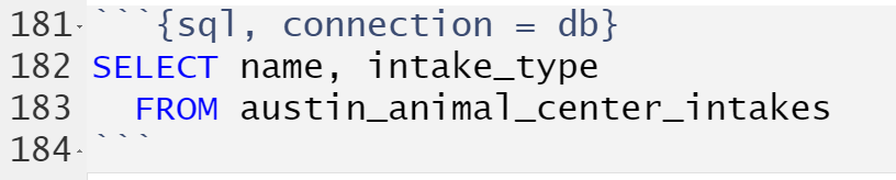
The above code chunk executes SQL code. So far, all our code chunks have had {r} at the beginning in order to indicate that R code is being used. However, this code chunk has {sql, connection = db} at the beginning to indicate that SQL code accessed through the database connection assigned to db is being used. Here is a picture of the code chunk as it appears within R Markdown.
This returns the two requested variables from the
austin_animal_center_intakes dataset.
Since * serves as a wildcard in SQL, use SELECT * FROM austin_animal_center_intakes to return all variables in the table.
A big difference between SQL commands and R commands is that SELECT and FROM are capitalized. Strictly speaking, this is not necessary, as SQL is case-insensitive, mainly because SQL was created in the days before it was common to allow upper and lower case within computer commands. That being said, the modern convention in SQL is to capitalize keywords like this. It turns out it helps greatly when reading the code to differentiate by case the functions from the parameters.
Suppose that it is necessary to rename one or more of the variables. Then the AS keyword to change things in the output.
| Name | Type |
|---|---|
| Scamp | Stray |
| Scamp | Public Assist |
| Bri-Bri | Stray |
| Tyson | Public Assist |
| Jo Jo | Public Assist |
| Oso | Owner Surrender |
| Oso | Public Assist |
| *Dottie | Stray |
| Manolo | Owner Surrender |
| Manolo | Owner Surrender |
This changes the name of the variables in the result to Name and Type
respectively.
For any variable with a space in its name, it is important to surround it with backticks so that it reads as one name.
| Name | Intake Type |
|---|---|
| Scamp | Stray |
| Scamp | Public Assist |
| Bri-Bri | Stray |
| Tyson | Public Assist |
| Jo Jo | Public Assist |
| Oso | Owner Surrender |
| Oso | Public Assist |
| *Dottie | Stray |
| Manolo | Owner Surrender |
| Manolo | Owner Surrender |
15.4 Unique values with DISTINCT
Consider only finding unique values of variables in a dataset. By adding the keyword DISTINCT to the SELECT command, different results are collapsed down (compare to unique.) For instance,
| animal_type |
|---|
| Dog |
| Cat |
| Other |
| Bird |
| Livestock |
Once it sees a value like "Dog", it no longer will return any observations that have "Dog" as the animal_type. From this, it appears that there are only five categories of animal in the database, Dog, Cat, Other, Bird, and Livestock.
Here is a more complicated query.
| animal_type | sex_upon_intake | age_upon_intake |
|---|---|---|
| Dog | Neutered Male | 10 years |
| Dog | Neutered Male | 7 years |
| Cat | Intact Female | 16 years |
| Dog | Neutered Male | 11 years |
| Dog | Spayed Female | 7 years |
| Dog | Intact Male | 3 years |
| Dog | Spayed Female | 2 years |
| Dog | Neutered Male | 9 years |
| Dog | Spayed Female | 1 year |
| Other | Unknown | 3 years |
There are 75947 animal records, but only 539 were returned. The very first line gives a Dog that is a Neutered Male with 10 years age upon intake. So further records with the same values will not be repeated in the returned output.
15.5 Using WHERE to filter observations
For R we used filter to pick out rows satisfying certain characteristics. For SQL, use WHERE to do the same thing.
For instance, suppose the output should be a list of all animals in the data set that are cats.
SELECT year, month, count, animal_type
FROM austin_animal_center_intakes_by_month
WHERE animal_type = "Cat"| year | month | count | animal_type |
|---|---|---|---|
| 2013 | 10 | 542 | Cat |
| 2013 | 11 | 436 | Cat |
| 2013 | 12 | 331 | Cat |
| 2014 | 1 | 335 | Cat |
| 2014 | 2 | 269 | Cat |
| 2014 | 3 | 353 | Cat |
| 2014 | 4 | 566 | Cat |
| 2014 | 5 | 901 | Cat |
| 2014 | 6 | 821 | Cat |
| 2014 | 7 | 881 | Cat |
Note that in SQL the logical equals operator is a single equals sign =, and not two equals signs as in most languages.
15.6 Arranging data using ORDER BY
The function arrange in the tidyverse puts rows in order by a specified column. In SQL, the command is called ORDER BY.
For instance,
SELECT year, month, count, animal_type
FROM austin_animal_center_intakes_by_month
WHERE animal_type = "Cat"
ORDER BY year, month| year | month | count | animal_type |
|---|---|---|---|
| 2013 | 10 | 542 | Cat |
| 2013 | 11 | 436 | Cat |
| 2013 | 12 | 331 | Cat |
| 2014 | 1 | 335 | Cat |
| 2014 | 2 | 269 | Cat |
| 2014 | 3 | 353 | Cat |
| 2014 | 4 | 566 | Cat |
| 2014 | 5 | 901 | Cat |
| 2014 | 6 | 821 | Cat |
| 2014 | 7 | 881 | Cat |
Unfortunately, the ordering for the second and subsequent terms in SQLite is alphabetical rather than numerical. So 2013 comes before 2014, but 11 comes before 3. When it is the only thing being used to order, it does things correctly.
SELECT year, month, count, animal_type
FROM austin_animal_center_intakes_by_month
WHERE animal_type = "Cat"
ORDER BY month| year | month | count | animal_type |
|---|---|---|---|
| 2014 | 1 | 335 | Cat |
| 2015 | 1 | 295 | Cat |
| 2016 | 1 | 304 | Cat |
| 2017 | 1 | 340 | Cat |
| 2014 | 2 | 269 | Cat |
| 2015 | 2 | 266 | Cat |
| 2016 | 2 | 279 | Cat |
| 2017 | 2 | 258 | Cat |
| 2014 | 3 | 353 | Cat |
| 2015 | 3 | 340 | Cat |
Descending order can be used by adding DESC to the command after the variable name.
SELECT year, month, count, animal_type
FROM austin_animal_center_intakes_by_month
WHERE animal_type = "Cat"
ORDER BY month DESC| year | month | count | animal_type |
|---|---|---|---|
| 2013 | 12 | 331 | Cat |
| 2014 | 12 | 341 | Cat |
| 2015 | 12 | 320 | Cat |
| 2016 | 12 | 419 | Cat |
| 2017 | 12 | 100 | Cat |
| 2013 | 11 | 436 | Cat |
| 2014 | 11 | 482 | Cat |
| 2015 | 11 | 488 | Cat |
| 2016 | 11 | 463 | Cat |
| 2017 | 11 | 427 | Cat |
15.7 NULL values and ORDER BY
The equivalent of NA in R is called NULL. By default, the ORDER BY command puts observations with a NULL value in the variable at the end of the list. To put these values first, add the helper function NULLS FIRST at the end of the ORDER BY line.
15.8 NULL values and logical operators
There are also logical operators in SQL, similar to those in R. The logical and is AND, logical or is OR, and logical not is NOT.
To look at data for cats where either the type was a stray or an owner surrender, use the following:
SELECT animal_type,
intake_type,
Intake_condition,
age_upon_intake
FROM austin_animal_center_intakes
WHERE animal_type = "Cat"
AND (intake_type = "Stray"
OR intake_type = "Owner Surrender")| animal_type | intake_type | intake_condition | age_upon_intake |
|---|---|---|---|
| Cat | Stray | Normal | 16 years |
| Cat | Stray | Normal | 1 month |
| Cat | Owner Surrender | Normal | 10 years |
| Cat | Owner Surrender | Normal | 9 months |
| Cat | Stray | Normal | 10 months |
| Cat | Owner Surrender | Sick | 15 years |
| Cat | Stray | Normal | 7 years |
| Cat | Stray | Normal | 3 years |
| Cat | Owner Surrender | Normal | 1 month |
| Cat | Owner Surrender | Normal | 1 month |
To deal with NULL
The equivalent of is.na is IS NULL.
The equivalent of
!is.nais IS NOT NULL.
For numerical data, to find observations with data value between two values, AND could be used, but there is also BETWEEN for this task.
SELECT year,
month,
animal_type,
COUNT
FROM austin_animal_center_intakes_by_month
WHERE count BETWEEN 901 AND 2000
ORDER BY month| year | month | animal_type | count |
|---|---|---|---|
| 2014 | 5 | Cat | 901 |
| 2014 | 5 | Dog | 966 |
| 2015 | 5 | Cat | 1009 |
| 2015 | 5 | Dog | 988 |
| 2016 | 5 | Cat | 921 |
| 2016 | 5 | Dog | 1020 |
| 2017 | 5 | Cat | 914 |
| 2015 | 6 | Cat | 1103 |
| 2015 | 6 | Dog | 1014 |
| 2014 | 7 | Dog | 926 |
Notice that the endpoints of the interval, 901 and 2000 will return true for BETWEEN 901 and 2000.
15.9 Transforming data
There are SQL commands for transforming the data before outputting it to the user. For operations that mutate was used for, just put the formula into SELECT. For example, to convert the age_in_days variable to age_in_years, use the following query.
SELECT monthyear,
animal_type,
outcome_type,
(age_in_days / 365) AS age_in_years
FROM austin_animal_center_age_at_outcome| monthyear | animal_type | outcome_type | age_in_years |
|---|---|---|---|
| 2014-03 | Dog | Return to Owner | 6.668493 |
| 2014-12 | Dog | Return to Owner | 7.454795 |
| 2015-11 | Cat | Return to Owner | 16.252055 |
| 2015-03 | Dog | Return to Owner | 11.972603 |
| 2015-04 | Dog | Return to Owner | 7.638356 |
| 2014-09 | Dog | Return to Owner | 2.668493 |
| 2014-01 | Dog | Euthanasia | 2.002740 |
| 2014-01 | Cat | Euthanasia | 15.013699 |
| 2014-01 | Dog | Return to Owner | 3.005479 |
| 2014-01 | Dog | Return to Owner | 2.013699 |
To round the year down to the nearest integer (as is usually done for ages that are given in years), use cast as int.
SELECT monthyear,
animal_type,
outcome_type,
cast(age_in_days / 365 as int) AS age_in_years
FROM austin_animal_center_age_at_outcome| monthyear | animal_type | outcome_type | age_in_years |
|---|---|---|---|
| 2014-03 | Dog | Return to Owner | 6 |
| 2014-12 | Dog | Return to Owner | 7 |
| 2015-11 | Cat | Return to Owner | 16 |
| 2015-03 | Dog | Return to Owner | 11 |
| 2015-04 | Dog | Return to Owner | 7 |
| 2014-09 | Dog | Return to Owner | 2 |
| 2014-01 | Dog | Euthanasia | 2 |
| 2014-01 | Cat | Euthanasia | 15 |
| 2014-01 | Dog | Return to Owner | 3 |
| 2014-01 | Dog | Return to Owner | 2 |
15.10 LIKE and NOT LIKE
There are many breeds of dogs in the observations.
SELECT sex_upon_outcome,
outcome_type,
outcome_subtype,
breed
FROM austin_animal_center_outcomes
WHERE animal_type = "Dog"
ORDER BY monthyear| sex_upon_outcome | outcome_type | outcome_subtype | breed |
|---|---|---|---|
| Spayed Female | Euthanasia | Aggressive | Labrador Retriever Mix |
| Neutered Male | Return to Owner | NA | Labrador Retriever |
| Neutered Male | Adoption | NA | Basset Hound |
| Neutered Male | Return to Owner | NA | Bullmastiff Mix |
| Neutered Male | Return to Owner | NA | Cocker Spaniel Mix |
| Spayed Female | Return to Owner | NA | Pit Bull Mix |
| Spayed Female | Return to Owner | NA | Pug |
| Spayed Female | Return to Owner | NA | Blue Lacy Mix |
| Spayed Female | Return to Owner | NA | Labrador Retriever Mix |
| Spayed Female | Return to Owner | NA | Pit Bull Mix |
Suppose the goal is to return only those observations where "wolfhound" appears somewhere in the breed name. The LIKE command can be used for this purpose.
There are two wildcards for this form of pattern matching. The first is the percent symbol %, which stands for any number of characters. This is equivalent to .* in regular expressions. The other wildcard character is the underscore _ which matches any single character. This is . in regular expressions.
Since the interest is in finding "wolfhound" anywhere in the breed, %wolfhound% will be the pattern searched for.
SELECT sex_upon_outcome,
outcome_type,
outcome_subtype,
breed
FROM austin_animal_center_outcomes
WHERE animal_type = "Dog" AND
breed LIKE "%wolfhound%"
ORDER BY monthyear| sex_upon_outcome | outcome_type | outcome_subtype | breed |
|---|---|---|---|
| Neutered Male | Transfer | Partner | Irish Terrier/Irish Wolfhound |
| Spayed Female | Adoption | NA | Irish Wolfhound Mix |
| Neutered Male | Transfer | Partner | Irish Wolfhound/Great Pyrenees |
| Neutered Male | Adoption | NA | Irish Wolfhound Mix |
| Neutered Male | Adoption | NA | Catahoula/Irish Wolfhound |
| Intact Female | Return to Owner | NA | Irish Wolfhound/Great Dane |
| Neutered Male | Transfer | Partner | Irish Wolfhound/Australian Shepherd |
| Neutered Male | Return to Owner | NA | Irish Wolfhound Mix |
| Intact Male | Return to Owner | NA | Irish Wolfhound Mix |
| Intact Female | Transfer | Partner | Irish Wolfhound Mix |
This matched six different breeds, and again ignored capitalization.
15.11 OFFSET
For a table that is very large, a query could take a very large amount of time. The LIMIT keyword limits the number of results obtained in the output.
SELECT DISTINCT animal_type,
        sex_upon_intake,
        age_upon_intake
  FROM austin_animal_center_intakes
LIMIT 7| animal_type | sex_upon_intake | age_upon_intake |
|---|---|---|
| Dog | Neutered Male | 10 years |
| Dog | Neutered Male | 7 years |
| Cat | Intact Female | 16 years |
| Dog | Neutered Male | 11 years |
| Dog | Spayed Female | 7 years |
| Dog | Intact Male | 3 years |
| Dog | Spayed Female | 2 years |
15.12 Using OFFSET
To give LIMIT the same power as slice, the OFFSET keyword can be used to skip the first few observations.
The following code skips the first 10 observations, then returns the next 7, so observations 11 through 17 are output.
| found_location | intake_type |
|---|---|
| Austin (TX) | Owner Surrender |
| 1111 W 34Th St in Austin (TX) | Public Assist |
| 12705 Lamplight Village in Austin (TX) | Wildlife |
| 6103 Manor Rd in Austin (TX) | Stray |
| 2318 Post Oak Rd. in Travis (TX) | Stray |
| Stassney & Westgate in Austin (TX) | Stray |
| 12900 Carillon Way in Manor (TX) | Stray |
15.13 SQL versus the tidyverse
Our commands so far.
| SQL | tidyverse |
|---|---|
| SELECT | select |
| WHERE | filter |
| ORDER BY | arrange |
| DESC | desc |
| NULL | NA |
| = | == |
| AND | & |
| NOT | ! |
| IS NULL | is.na |
| IS NOT NULL | !is.na |
| LIMIT and OFFSET | slice |
Now that the chapter is finished, disconnect from our database connection with dbDisconnect.
Questions
Suppose that the USArrests dataset was in an SQL database.
| State | Murder | Assault | UrbanPop | Rape |
|---|---|---|---|---|
| Alabama | 13.2 | 236 | 58 | 21.2 |
| Alaska | 10.0 | 263 | 48 | 44.5 |
| Arizona | 8.1 | 294 | 80 | 31.0 |
| Arkansas | 8.8 | 190 | 50 | 19.5 |
| California | 9.0 | 276 | 91 | 40.6 |
| Colorado | 7.9 | 204 | 78 | 38.7 |
Create an SQL query for this dataset that returns the state, murder rate, and assault rate for those states that have a murder rate of at least 10.
Create an SQL query for this dataset that returns the state, murder rate, and assault rate for those states that have a murder rate of at least 10 and at most 15.
Suppose that the iris dataset was in an SQL database.
| Sepal.Length | Sepal.Width | Petal.Length | Petal.Width | Species |
|---|---|---|---|---|
| 5.1 | 3.5 | 1.4 | 0.2 | setosa |
| 4.9 | 3.0 | 1.4 | 0.2 | setosa |
| 4.7 | 3.2 | 1.3 | 0.2 | setosa |
| 4.6 | 3.1 | 1.5 | 0.2 | setosa |
| 5.0 | 3.6 | 1.4 | 0.2 | setosa |
| 5.4 | 3.9 | 1.7 | 0.4 | setosa |
Write an SQL query for the iris SQL database that does the following:
Sorts the observations by order of the petal width in descending order.
Keeps only the top five observations.
Returns the petal length, petal width, and species data for these observations.
Suppose the PlantGrowth dataset built in to R was in an SQL database.
| weight | group |
|---|---|
| 4.17 | ctrl |
| 5.58 | ctrl |
| 5.18 | ctrl |
| 6.11 | ctrl |
| 4.50 | ctrl |
| 4.61 | ctrl |
Write an SQL query that finds the unique values that
grouptakes on.Write an SQL query that only keeps observations where the
groupis"ctrl".Write an SQL query that only keeps observations where the
groupis"ctrl"and the weight is at least 5.
Suppose that a relational database has two tables. The first table Territory has variables State, Level, Capital, and the second table Region has variables State, Mining, and Population.
Write SQL code to return the variables
StateandLevelfromTerritory.Write SQL code to return the variable
MiningFromRegion, but renamed toMine Output.
Suppose that the relational database includes a table Region has variables State, Mining, and Population. The Mining variable is either high, med, or low.
Write SQL code that accomplishes the following.
Removes all observations where the population is less than one million.
Orders the remaining observations in decreasing order of population.