Foundations of Data Science
2026-01-20
1 Introduction to Data Science
Summary
A data scientist can get data into an effective computer readable form, learn about the data through transformation, visualization, and modeling, and communicate their results to the outside world.
R is a statistical programming language.
An Integrated Development Environment (IDE) is a set of tools for working with a programming language effectively.
RStudio is an IDE for R that allows us to easily use R through the console, scripts, and R Markdown.
The term data science is a relatively recent addition to the English language, going back about seventy years. But data and its collection is nearly as old as humans themselves, going back to our first attempts as humans to learn about the world around us. For instance, forty thousand years ago people used tally marks to record numbers. These developed into symbols and true written languages around five thousand years ago, and ever since humans have been recording events and observations in order to improve their lives.
In the past, gathering data was a painstaking process, but recent growth in the use of the Internet (which is estimated at 7 billion users) coupled with the ability to take digital photos and video, has resulted in a huge data intake. In 2021, estimates are that between 2.5 and 4.5 exabytes of information are created every day on Earth. Exa is the metric prefix for \(10^{18}\), or a million million million.
Those exabytes are then stored on hard disks, flash drives, and in cloud-based servers around the world, and all of this data is being collected and analyzed by computers to determine patterns and correlations in it. This is data science.
The analysis of these datasets allows corporations and governments to make better decisions about such things as marketing, supply chains, and disaster planning. Data science is not a new field, but it has exploded in recent years, and the demand for data scientists is at an all time high.
1.1 What is data science?
Data consist of observations recorded for later use.
Why is collecting and recording data so important? Typically the purpose is to try and answer a particular question or obtain some sort of knowledge from the data.
Data science consists of the methods and tools for collecting and studying data, with a goal of making informed decisions.
Modern data science requires modern tools, and much of data science today involves understanding computation for datasets with a goal of making these computations as efficient as possible. That is why modern data science is often seen as being at the intersection of statistics whose tools are used to analyze data, and computer science whose tools are used to record and carry out the computations suggested by the analysts effectively.
Each dataset comes from a domain of knowledge. How the dataset is studied often depends on that domain. An analyst studying images on the web will have very different data from an economist studying time series data of interest rates. That is why the third piece (after statistics and computer science) of data science is domain knowledge, understanding data in the context of a specific discipline.
1.2 Tasks of DS
Even with all the many different types of data there are out there some common ideas apply in all situations. This allows us to break down the work of data scientists into basic tasks that face anyone working with data. Then the techniques for accomplishing these tasks based on the data type can be studied.
Getting data into a form that can be read easily by a computer and other humans.
Understand what the data is telling us.
Communicate what the data says to the rest of the world.
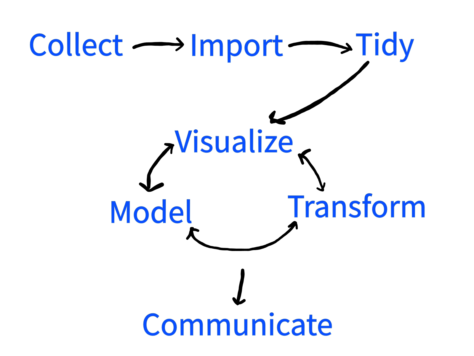
These can be divided further as follows.
The first step in a project is the collection of data. The time needed to get data can range from years to almost instantaneous depending on the application.
Once the data is collected, digital computers are the most effective tool for analyzing that data. The step of moving data recorded by a researcher into a computer for processing is called the import step.
There are certain conventions that are used throughout mathematics, statistics, and the sciences. For instance, given variables \(x\) and \(y\), the variable \(x\) is usually plotted on the horizontal axis, and \(y\) is plotted on the vertical. By using this convention, a writer makes it easier for their audience to understand new material.
In the same way, there is a standard way to format and present data. Putting the data into a form that follows these conventions is called tidying the data.
Once the data has been imported and tidied, next comes the task of understanding it. This takes on several different forms. Human brains are great at picking out visual patterns, and so a popular first step for understanding how data behaves is to use visualization tools.
Another aspect of understanding data is building a mathematical model of the data.
In order to make the tasks of visualization and modeling easier, often it is necessary to transform the data. This can involve picking out the most important parts, or projecting the data onto a plane or curve, or any activity that helps to make sense of the dataset.
These three activities are not done in isolation, but build off of each other. An early visualization might make a researcher realize that their data lies in a subspace of the available variables. By transforming the data by projecting onto that subspace, a new visualization might see further patterns that were hidden in the original data. A specific model might lead to a better visualization, which gives the user a transformation of the data that needs a new model. And so it goes, one technique feeding into the other until the complexities of the data is understood.
At this point the goal is to be able to communicate what the data has shown to the rest of the world, and communication is typically the final step in the process.
This can be summarized with the following diagram.
While the term Big Data has recently become popular, the datasets studied by statisticians have always been large, for instance census data from centuries ago could run into millions of observations.
Today, Big Data is considered to be any dataset that is impractical to bring within a single workstation. Because dealing with large datasets is so difficult, the methods needed for Big Data are often somewhat different than those used for smaller datasets. Still, the basic principles are the same, it is mostly the computer science aspects that change.
Because the capabilities of workstations are continually growing, what counts as Big Data is constantly changing as well. As computers grow in power, more and more datasets of large size can be handled effectively without specialized tools. The tools used in this text can be easily used on datasets with millions of observations.
1.3 R
The programming language for this text will be R. Most data science today is done in R, Python, Matlab, Java, and a few other languages. With proper package support, each is capable on its own of handling most data analysis tasks. R is a good place to start because the language has a console where commands can be tested directly, helping a user to build an intuitive understanding of the language. Moreover, R was designed from the ground up for statistical analyses.
R is a programming environment designed for statistical analysis.
The R language interpreter can be downloaded for free from https://cloud.r-project.org/ for Windows, Mac, and Linux. This text also uses an Integrated Development Environment (IDE) for R called RStudio. This IDE is also Open Source, and can be downloaded for free from https://www.rstudio.com/products/rstudio/download/.
An Integrated Development Environment (aka IDE) is a software program that brings together the tools you need to work with a programming environment effectively.
The most popular IDE for R is RStudio.
RStudio allows the user to easily switch between entering commands one-at-a-time, building up an ordered list of commands to form programs, viewing help, seeing graphical output, and organizing file structure. It helps make large projects manageable.
Primarily, we will be using R through RStudio using either the console, or an R Markdown file.
Console. You can type commands in R directly into the console as in Python or MATLAB.
R Markdown. A markup language uses tags to create a professional looking document. Markdown is a very simple document preparation system, and R Markdown allows the user to easily incorporate R code into their document. The code chunks inside can also be quickly transferred to the console and run. This makes this a notebook system as well. These files typically end in extension
.Rmd. This type of file will be described extensively in the next chapter.
1.4 Types of languages
Code is a term for the commands that we give to a computer.
Computer code (aka a computer program) is a set of instructions for a computing environment.
There are several types of computer languages. The most basic language is machine language which consists of commands that can be directly understood by a computer’s processor.
Machine language (aka machine code) consists of commands that can be directly understood by the processing unit of a computer.
In the early days of data science, machine language was used extensively, but today it is quite rare. The reason is the development of interpreted languages and compiled languages. Typically these languages are easy for humans to read. They require a method of translation into machine language so that the computer can understand them.
In a compiled language there exists a compiler that translates the program into machine readable code, which can then be run without the need for the compiler.
In an interpreted language, there is an interpreter which translates the program into machine code every single time the program is run. The program cannot be executed without the presence of the interpreter.
R is an interpreted language.
Both compiled and interpreted languages have several advantages over machine code. The biggest is that the same code can be interpreted/compiled to run on many different machines. This is why there is a Windows, MacOS, and Linux version of R. The same code can be used on any of these machines. Another advantage is readability. While the language of R is not quite English or mathematical symbolism, it is much closer to being directly readable by a person.
1.5 The R console
Interpreted languages lend themselves to the possibility of having a console.
A console, aka shell, aka command line interface (CLI), in an interpreted programming language accepts and executes commands one at a time.
When you first start RStudio, in the lower left corner will be the console. Before we put commands together to form programs, in the console you can try out commands individually. The preferred assignment operator in R is <-. As its name implies, it is used to assign values to variables. So for instance the commands
returns the output
## [1] 9The ## indicates that this line is output from the R interpreter. The [1] indicates that the output starts with the first number in the result. This is really only useful when the output has many numbers that take more than one line to print. The 9 is the actual result. Later on we will work with vectors where we might not start with the first number in our output.
Some variables are already defined in R. So for instance, if you type
into the console, it will give you all 50 lines of data from the cars dataset that is built into R. To get an idea of what is in this dataset without printing the whole thing, the head function can be used to just get the first few lines. A function is a command that can require inputs. These inputs are placed in parentheses, (), that come after the name of the function. For instance:
##   speed dist
## 1     4    2
## 2     4   10
## 3     7    4
## 4     7   22
## 5     8   16
## 6     9   10
calls the function head with the input cars. The head function gives by default the first 6 observations in the dataset. It also prints as the first line the headings for the columns of data, speed and dist.
The ? operator opens the help within R. Using
?carsin RStudio opens up the help in the lower right corner window (in the default setup) and tells us that this variable represents speed and stopping distance data for a number of cars from the 1920’s.
Another name for a function is command. Using the summary command on the cars dataset gives a basic statistical analysis.
##      speed           dist
##  Min.   : 4.0   Min.   :  2.00
##  1st Qu.:12.0   1st Qu.: 26.00
##  Median :15.0   Median : 36.00
##  Mean   :15.4   Mean   : 42.98
##  3rd Qu.:19.0   3rd Qu.: 56.00
##  Max.   :25.0   Max.   :120.00
There are two types of functions, mathematical functions (also called pure functions) whose output only depends on the input, and programming functions whose output might depend on other things besides what is input.
A statistic is any mathematical function of the data.
The cars data summary, reveals (among other things) that the minimum speed value among all the cars is 4.0. It also gives the sample mean, which is the sum of the values divided by the number of values. This is 15.4. The mean is an example of a measure of central tendency, and is one indication of where the center of the data lies.
The sample average of values \(x_1,\ldots,x_n\) is \[ \bar x = \frac{x_1+\cdots+x_n}{n}. \]
From the summary, the sample average of the speed of the cars is 15.4, and the average of the stopping time is 42.98. What these statistics do not tell is how the speed and stopping distance are related.
To understand this, it is helpful to have a way of visualizing the relationship.
The simplest thing is to make a plot of the distance values versus the speed values. The plot and $ operators can do just that. (Later on, a more systematic way of constructing plots will be presented. For now, though, the basic built in commands to R will suffice.)
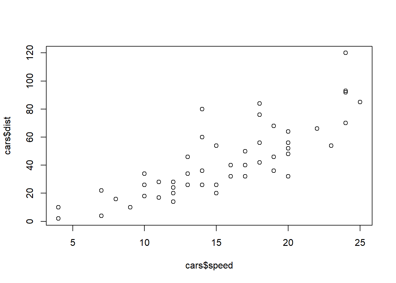
The beauty of a visualization like this is that it immediately makes apparent the relationship between the speed and the stopping distance: as the car goes faster, the stopping distance tends to be greater.
Questions
True or False: Recording the temperature for a city for a week is creating data that can be used to adjust power station output.
True or False: Data Science studies using data to make informed decisions.
Name seven tasks that data scientists do.
What was the programming environment R designed to do?
Is it necessary to use an IDE when programming in a particular language?
A set of instructions for a computer is often called a computer program, also known as what?
What is the term for commands that can be directly understood by a computer?
Is R an interpreted or complied language?
Find by hand the sample average of \(3.2, 4.1,\) and \(2.6\).