8 Grouping observations
Summary
The group_by function tells R to partition the observations into one or more groups based on any variable. This changes the workings of summarize, filter, and mutate.
Calculating the mean of a variable in a tibble can be done with summarize. When grouped, this function performs its action within each group.
Any mean or similar function applied to a grouped tibble will for purposes of filter and mutate will do the filtering or calculate the function only on observations within each group.
Applying ungroup to a tibble will remove a grouping. The application of summarize will also run the ungroup function on the dataset.
The rank function assigns to each observation based on a variable input, the smallest value 1, the next smallest 2, and so on. Ties can then be resolved in a variety of ways.
8.1 Counting group type
Consider the transit revenue data from earlier, available from https://s3.us-west-1.amazonaws.com/markhuber-datascience-resources.org/Data_sets/Transit_Operators_-_Revenues.csv.
## Rows: 196218 Columns: 11
## ── Column specification ───────────────────────────────────
## Delimiter: ","
## chr (8): Entity Name, Type, Form/Table, Category, Subcategory, Line Descript...
## dbl (3): Fiscal Year, Value, Row Number
##
## ℹ Use `spec()` to retrieve the full column specification for this data.
## ℹ Specify the column types or set `show_col_types = FALSE` to quiet this message.
The largest year in the data is 2021. Note that Fiscal Year was surrounded by backticks because the variable name contains a space.
## # A tibble: 6 × 2
##   `Fiscal Year` `City, State`
##           <dbl> <chr>
## 1          2021 Arcadia, CA
## 2          2021 Arcadia, CA
## 3          2021 Arcadia, CA
## 4          2021 Arcadia, CA
## 5          2021 Wasco, CA
## 6          2021 Wasco, CA
The smallest year in the data is 2003.
## # A tibble: 6 × 2
##   `Fiscal Year` `City, State`
##           <dbl> <chr>
## 1          2003 Marysville, CA
## 2          2003 Marysville, CA
## 3          2003 Marysville, CA
## 4          2003 Marysville, CA
## 5          2003 Marysville, CA
## 6          2003 Marysville, CA
So a simple question: how many observations are there from each year? For visualizations, the geom_bar can be used to break the observations by Fiscal Year, and then count each one.
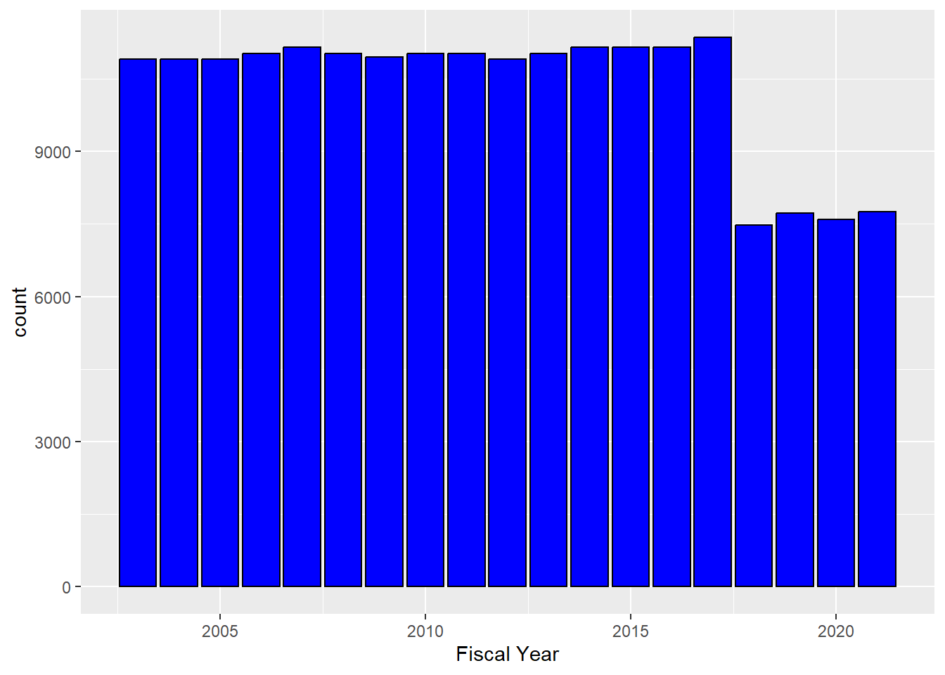
Interesting: the numbers were stable until 2017, but in 2018 there was a drop. Tax law change? Other legislation? In any event, it would be nice to have the exact numbers.
The n function within summarize can tell the number of observations in a dataset.
## # A tibble: 1 × 1
##    `n()`
##    <int>
## 1 196218
Okay, so that is the total number of entries in the dataset. To get this broken down year by year, one could start filtering the dataset by year and summarize at each step.
## # A tibble: 1 × 1
##   count
##   <int>
## 1 10906## # A tibble: 1 × 1
## count
## <int>
## 1 10906This gets pretty tedious fast, though.
A better way is to partition the observations of the dataset into one or more groups. This can be done with the group_by.
## # A tibble: 196,218 × 11
## # Groups:   Fiscal Year [19]
##    `Entity Name`     `Fiscal Year` Type  `Form/Table` Category
##    <chr>                     <dbl> <chr> <chr>        <chr>
##  1 Access Services …          2017 Reve… TO_INCOME_S… Operati…
##  2 Access Services …          2017 Reve… TO_INCOME_S… Operati…
##  3 Access Services …          2017 Reve… TO_INCOME_S… Operati…
##  4 Access Services …          2017 Reve… TO_INCOME_S… Operati…
##  5 Access Services …          2017 Reve… TO_INCOME_S… Operati…
##  6 Access Services …          2017 Reve… TO_INCOME_S… Operati…
##  7 Access Services …          2017 Reve… TO_INCOME_S… Operati…
##  8 Access Services …          2017 Reve… TO_INCOME_S… Operati…
##  9 Access Services …          2017 Reve… TO_INCOME_S… Operati…
## 10 Access Services …          2017 Reve… TO_INCOME_S… Operati…
## # ℹ 196,208 more rows
## # ℹ 6 more variables: Subcategory <chr>,
## #   `Line Description` <chr>, Value <dbl>,
## #   `City, State` <chr>, `Zip Code` <chr>, `Row Number` <dbl>
At first, this command does not look like it does anything! All of the 196218 observations are still there. What it has done is to break the observations into 19 different groups. The first group has fiscal year 2003, the next 2004, and so on up to 2021. Any commands which follow this one will be applied to each of these 19 groups separately.
So if the next command is summarize(count = n()), then this command is applied to the 2003 group, the 2004 group, the 2005 group, and so on up to the 2021 group. That is a lot of work saved. Moreover, once the command is done, it takes all 19 results, and puts them together in a tibble, with one column that is the variable that the grouping was done by, and one variable that returns the results.
Whew, so after all that is done, the result looks something like this.
## # A tibble: 19 × 2
##    `Fiscal Year` count
##            <dbl> <int>
##  1          2003 10906
##  2          2004 10906
##  3          2005 10906
##  4          2006 11029
##  5          2007 11152
##  6          2008 11029
##  7          2009 10947
##  8          2010 11029
##  9          2011 11029
## 10          2012 10906
## 11          2013 11029
## 12          2014 11152
## 13          2015 11152
## 14          2016 11152
## 15          2017 11357
## 16          2018  7479
## 17          2019  7722
## 18          2020  7587
## 19          2021  7749
To reiterate, the group_by(Fiscal Year) line means there will be a group for Fiscal Year 2003, 2004, and so on up to 2021. The summarize(count = n()) line means that for each group, the n function will be applied to count how many observations are in each group. Finally, the result is put back together into a tibble.
8.1.1 Multiple groups
It is possible to group on more than one variable. For instance, if the data is grouped first by year, and then by city, then summarize(n()) will count the number of observations with each possible year-city pair.
## `summarise()` has grouped output by 'Fiscal Year'. You can
## override using the `.groups` argument.
## # A tibble: 3,150 × 3
## # Groups: Fiscal Year [19]
## `Fiscal Year` `City, State` count
## <dbl> <chr> <int>
## 1 2003 Alameda, CA 41
## 2 2003 Albany, CA 41
## 3 2003 Alhambra, CA 82
## 4 2003 Alturas, CA 41
## 5 2003 Antioch, CA 82
## 6 2003 Arcadia, CA 41
## 7 2003 Arcata, CA 41
## 8 2003 Arroyo Grande, CA 41
## 9 2003 Arvin, CA 41
## 10 2003 Atascadero, CA 41
## # ℹ 3,140 more rows8.1.2 Summarizing means
The iris dataset is built into R, and measures the petal and sepal length for 150 flowers from three species.
##   Sepal.Length Sepal.Width Petal.Length Petal.Width Species
## 1          5.1         3.5          1.4         0.2  setosa
## 2          4.9         3.0          1.4         0.2  setosa
## 3          4.7         3.2          1.3         0.2  setosa
## 4          4.6         3.1          1.5         0.2  setosa
## 5          5.0         3.6          1.4         0.2  setosa
## 6          5.4         3.9          1.7         0.4  setosa
There are three different species covered by the dataset.
##        Species
## 1       setosa
## 51  versicolor
## 101  virginica
As before, the number of observations from each species can be found with the n function.
## # A tibble: 3 × 2
##   Species    count
##   <fct>      <int>
## 1 setosa        50
## 2 versicolor    50
## 3 virginica     50
The sample average of the petal length can also be found for each species.
## # A tibble: 3 × 3
##   Species    count mean_petal_length
##   <fct>      <int>             <dbl>
## 1 setosa        50              1.46
## 2 versicolor    50              4.26
## 3 virginica     50              5.55
8.2 Grouping with filter
These groups also work with the logical expressions in filter.
For instance,
## # A tibble: 30,537 × 11
## # Groups:   Fiscal Year [4]
##    `Entity Name`     `Fiscal Year` Type  `Form/Table` Category
##    <chr>                     <dbl> <chr> <chr>        <chr>
##  1 Arcadia                    2021 Reve… Statement o… Nonoper…
##  2 Arcadia                    2021 Reve… Statement o… Nonoper…
##  3 Arcadia                    2021 Reve… Statement o… Nonoper…
##  4 Access Services …          2019 Reve… Statement o… Operati…
##  5 Arcadia                    2021 Reve… Statement o… Nonoper…
##  6 Wasco                      2021 Reve… Statement o… Nonoper…
##  7 Wasco                      2021 Reve… Statement o… Nonoper…
##  8 Wasco                      2021 Reve… Statement o… Nonoper…
##  9 Arcadia                    2021 Reve… Statement o… Nonoper…
## 10 Arcadia                    2021 Reve… Statement o… Nonoper…
## # ℹ 30,527 more rows
## # ℹ 6 more variables: Subcategory <chr>,
## #   `Line Description` <chr>, Value <dbl>,
## #   `City, State` <chr>, `Zip Code` <chr>, `Row Number` <dbl>
only keeping observations from those years where the number of observations in that year was at most 10000.
In the iris data, suppose only flowers with average petal length of at least 5 are desired.
## # A tibble: 50 × 5
## # Groups:   Species [1]
##    Sepal.Length Sepal.Width Petal.Length Petal.Width Species
##           <dbl>       <dbl>        <dbl>       <dbl> <fct>
##  1          6.3         3.3          6           2.5 virginica
##  2          5.8         2.7          5.1         1.9 virginica
##  3          7.1         3            5.9         2.1 virginica
##  4          6.3         2.9          5.6         1.8 virginica
##  5          6.5         3            5.8         2.2 virginica
##  6          7.6         3            6.6         2.1 virginica
##  7          4.9         2.5          4.5         1.7 virginica
##  8          7.3         2.9          6.3         1.8 virginica
##  9          6.7         2.5          5.8         1.8 virginica
## 10          7.2         3.6          6.1         2.5 virginica
## # ℹ 40 more rows
Since only the virginica species satisfies this criterion, this is the only group in Species represented in the output.
8.3 Grouping with mutate
In the iris data set, the average Petal.Length was different for each species.
iris |>
  select(Petal.Length, Species) |>
  group_by(Species) |>
  summarize(mean_petal_length = mean(Petal.Length))
## # A tibble: 3 × 2
## Species mean_petal_length
## <fct> <dbl>
## 1 setosa 1.46
## 2 versicolor 4.26
## 3 virginica 5.55One type of calculation often needed is for each observation, what is the length compared to the average length? In other words what is Petal.Length divided by mean(Petal.Length) for each observation, where the mean is with respect to the Species? Here mutate is helpful, remembering that a command like mean will be applied only to those observations in the group.
iris |>
  select(Petal.Length, Species) |>
  group_by(Species) |>
  mutate(rel_petal_length = Petal.Length / mean(Petal.Length))
## # A tibble: 150 × 3
## # Groups: Species [3]
## Petal.Length Species rel_petal_length
## <dbl> <fct> <dbl>
## 1 1.4 setosa 0.958
## 2 1.4 setosa 0.958
## 3 1.3 setosa 0.889
## 4 1.5 setosa 1.03
## 5 1.4 setosa 0.958
## 6 1.7 setosa 1.16
## 7 1.4 setosa 0.958
## 8 1.5 setosa 1.03
## 9 1.4 setosa 0.958
## 10 1.5 setosa 1.03
## # ℹ 140 more rows8.4 Using rank
One common task is to rank data from smallest to largest. For instance, consider the following.
## [1] 3 1 2Here 4.6 is the third smallest number, 1.4 is the first smallest number, and 1.6 is the second smallest number. When there are ties, the ranks given (by default) are the average ranks.
## [1] 2.5 2.5 1.0To change this behavior, the ties.method parameter can be changed. The "min" behavior works like in sports or the U.S. News and World report college rankings, where every tie shares in the highest possible place.
## [1] 2 2 1Note that if there is a tie for first place, the next available place is third place.
## [1] 3 3 1 1Suppose that given the iris data, the goal is to find the observations with rank less than 3 using minimum rank for longest petal length. The rank function together with filter can be used to make this happen.
##   Sepal.Length Sepal.Width Petal.Length Petal.Width Species
## 1          4.3         3.0          1.1         0.1  setosa
## 2          4.6         3.6          1.0         0.2  setosa
Now suppose the idea is to find the observations associated with the two longest petal lengths for each of the species. Again, group_by effectively turns the one dataset into three datasets, one for each species.
## # A tibble: 8 × 5
## # Groups:   Species [3]
##   Sepal.Length Sepal.Width Petal.Length Petal.Width Species
##          <dbl>       <dbl>        <dbl>       <dbl> <fct>
## 1          4.3         3            1.1         0.1 setosa
## 2          4.6         3.6          1           0.2 setosa
## 3          4.9         2.4          3.3         1   versicolor
## 4          5           2.3          3.3         1   versicolor
## 5          5.1         2.5          3           1.1 versicolor
## 6          4.9         2.5          4.5         1.7 virginica
## 7          6.2         2.8          4.8         1.8 virginica
## 8          6           3            4.8         1.8 virginica
There are only three observations for versicolor and virginica that fit the bill because there is a tie for second place for these flowers.
8.5 Ungrouping
If there is a need to get rid of a group structure, use the function ungroup. This returns the tibble to its original form.
Note that after using grouping and a summarize command, each row is an observation that is a single group. Therefore, there is typically no need for a group structure, and ungroup is automatically applied.
Questions
The following question is in reference to the transit revenue dataset transrev used above.
Write code to count the number of observations for each city in California.
Write code to keep only observations from cities that have more than 50 observations in a given year.
In the flights data set, the variable tailnum tells us the exact plane that took a flight.
Find the plane that flew the most number of the flights.
How many planes flew at least 100 flights?
Which carrier had the highest percentage of on-time flights?