21 Machine learning
Summary
Machine learning is the term for algorithms that learn from the data how to build a model. Previously, lm and cforest were introduced for making models, but there are hundreds more such functions.
rlm creates a robust linear model that is less sensitive to outliers.
svm creates a support vector machine model.
glm creates generalized linear models. In particular, with parameter setting
family = "binomial", this can do logistic regression.
21.1 What is machine learning?
Machine learning is the area of computer science that deals with algorithms designed to learn from datasets how to accomplish various tasks.
A good machine learning algorithm will improve its results as more data is fed into the system. Often it is said that the algorithms gain experience, or learn from the data. There are still models in machine learning, but they are designed to be much more flexible than the classic linear models. Often machine learning algorithms go beyond just fitting parameters to deciding the more basic question of which factors serve as the best predictor variables in the first place.
The four main tasks of machine learning are the following.
Classification Here the response is a categorical variable with a finite set of possibilities. The goal is to know which possible outcome is the best class for our observation.
Prediction This applies when our response is numerical. Here the goal is usually to minimize some measure of how far away the prediction is from the true answer.
Density estimation Often observations do not have factors spread over all possible values, but instead concentrate on a particular area. The goal here is to understand where the density of input values is highest.
Pattern recognition Observations are often very high dimensional. For instance, a photograph might have 16 million pixels. A 16 million dimensional model is too much to handle for classical methods! Instead, we look for lower dimensional behavior within the set of models. This allows us to project the data onto a much lower dimensional data set.
There are two types of machine learning.
In supervised learning there is a training set that has labeled data. For each set of possible predictors, the output is known in the training set.
This is the type of machine learning used in the Titanic survival case study.
In unsupervised learning there is no labeled dataset. The goal is to learn about the data solely from the data values themselves.
Some common methods for supervised learning include:
Decision Trees and Random Forests
Linear Regression
Logistic Regression
Boosting
Support Vector Machines
Bayesian Classifiers/Bayesian Networks
Neural Networks
Deep learning
Some common methods for unsupervised learning include:
Clustering
Anomaly detection
Topic modeling
Neural Networks
21.2 Supervised learning
Here a few of these methods are considered in more detail.
21.2.1 Decision Trees and Random Forests
In this method, the goal is to split the state space of inputs into two equal parts, where the values of the response variable are similar within each part.
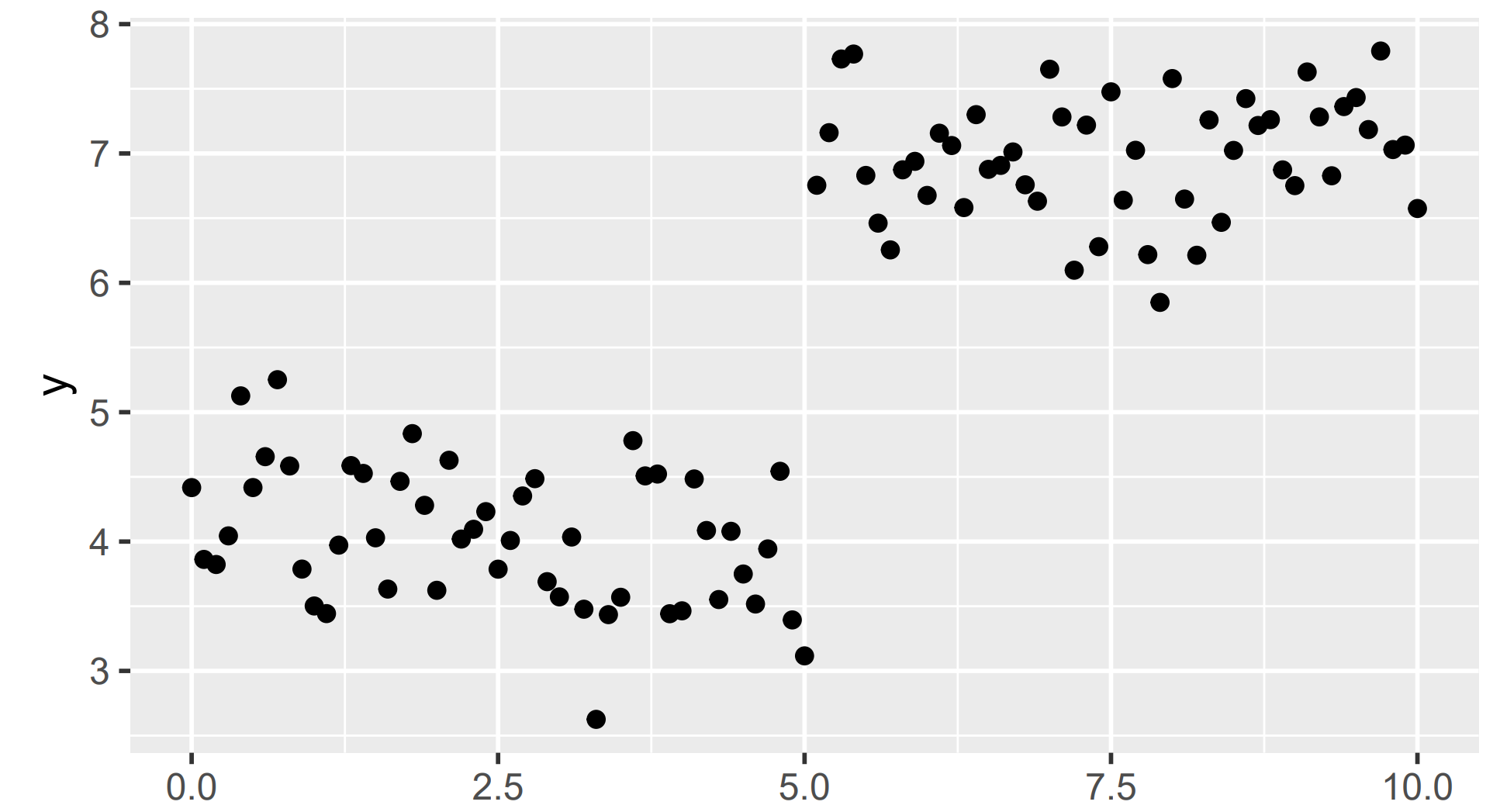
In the data above, there is a clear break in the \(y\) values for \(x < 5\) and \(x \geq 5\). On either side of this split, the \(y\) values are much closer to one another.
Each node of a decision tree breaks the input space into two pieces where the response is closer to its center in each of the two trees than in the overall space.
In the toy example above, the decision tree idea works very well. Unfortunately, in real data this method can be prone to overfitting. To solve this problem, a random forest works by performing the decision tree process multiple times. Each time a tree is created, a bit of randomness is intentionally injected into the tree process.
The set of trees together is called a random forest. When a user then inputs a new observation and wants a prediction of the response, each tree is run separately. The final result can then be found by looking at the level most commonly seen for categorical response, or the average of the predictions from each tree for a numerical response.
A random forest is a collection of decision trees where at each step in their formation, some random choices were made.
It is well known that a survey of a group of individuals can sometimes perform better than a single expert on a topic. Each individual member of the group has less information about the subject, but some are biased high and some are biased low as to the true answer. By averaging their information, the result is often better than a single person whose biases are unknown. This phenomenon sometimes goes by the name wisdom of the crowd.
In the same way, each individual decision tree in the random forest might be biased towards some response or another based on how it was created. However, since the process has been done randomly multiple times, some trees will be biased in a certain way while some trees will be biased in the opposite way. Together their average is close to the true value.
21.2.2 Linear regression
The nice thing about random forests is that we need to know very little about the structure of the data in order to make accurate predictions. If we do know more about the structure of the data, then a linear regression model might be in order.
For instance, consider the following randomly generated data set.
x <- seq(from = 0, to = 10, by = 0.1)
y2 <- 3 + x + rnorm(length(x), 0, 0.5)
tibble(x, y2) |>
  ggplot(aes(x, y2)) +
    geom_point()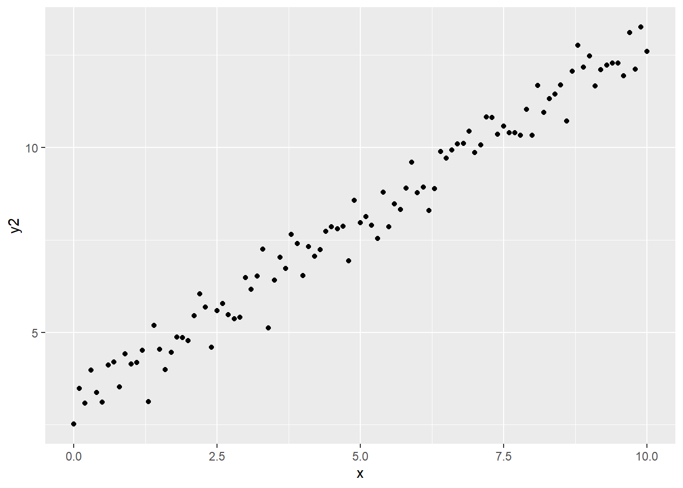
A decision tree would have to break this down into many pieces to get an accurate read, while a simple linear model does better with only a slope parameter and \(y\)-intercept parameters.
Suppose we have \(n\) observations and \(p\) predictor variables. Call the column vector of the response variable values \(Y\). Then form a model matrix whose \(i,(j+1)\)th entry is the value of the \(j\)th predictor variable in the \(i\)th observation, and whose \(i, 1\) entry is always 1. Then the model \[ Y = X\beta + \epsilon, \] where \(Y\) is an \(n\) by 1 matrix, \(X\) is an \(n\) by \(p + 1\) matrix, \(\beta\) is a \(p + 1\) by \(1\) matrix, and \(\epsilon\) is an \(n\) by 1 matrix. This is called a linear model of the data, and the \(\beta\) values are called the parameters of the model.
One reason that linear models are widely used is that if our goal is to minimize the sum of the squares of the \(\epsilon\) values, it is possible to solve for the \(\beta\) values exactly given \(Y\) and \(X\). If there are many observations and predictors, these computations can still take a long time, however, it is still possible to approximate the values of \(\beta\) that is the best fit.
21.2.3 Logistic regression
Linear models do better with numerical data and decision trees do better with categorical data. Is there a way to use linear models for categorical data? Consider the best least squares fit for the following data where the response is either 0 or 1.
First consider generating some random 0-1 data. The data has a 10% chance of being 1 if x is at most 5, and a 90% chance of being 1 if x is greater than 5.
A regular linear model tries to put a straight line through this cloud of points! First create the linear model
Next, the modelr will be used.
Now create the predictions.
df3 <- tibble(x, y3)
df3_pred <- df3 |>
add_predictions(mod1)
ggplot() +
geom_point(data = df3, aes(x, y3)) +
geom_line(data = df3_pred, aes(x, pred), color = "red", lwd = 1)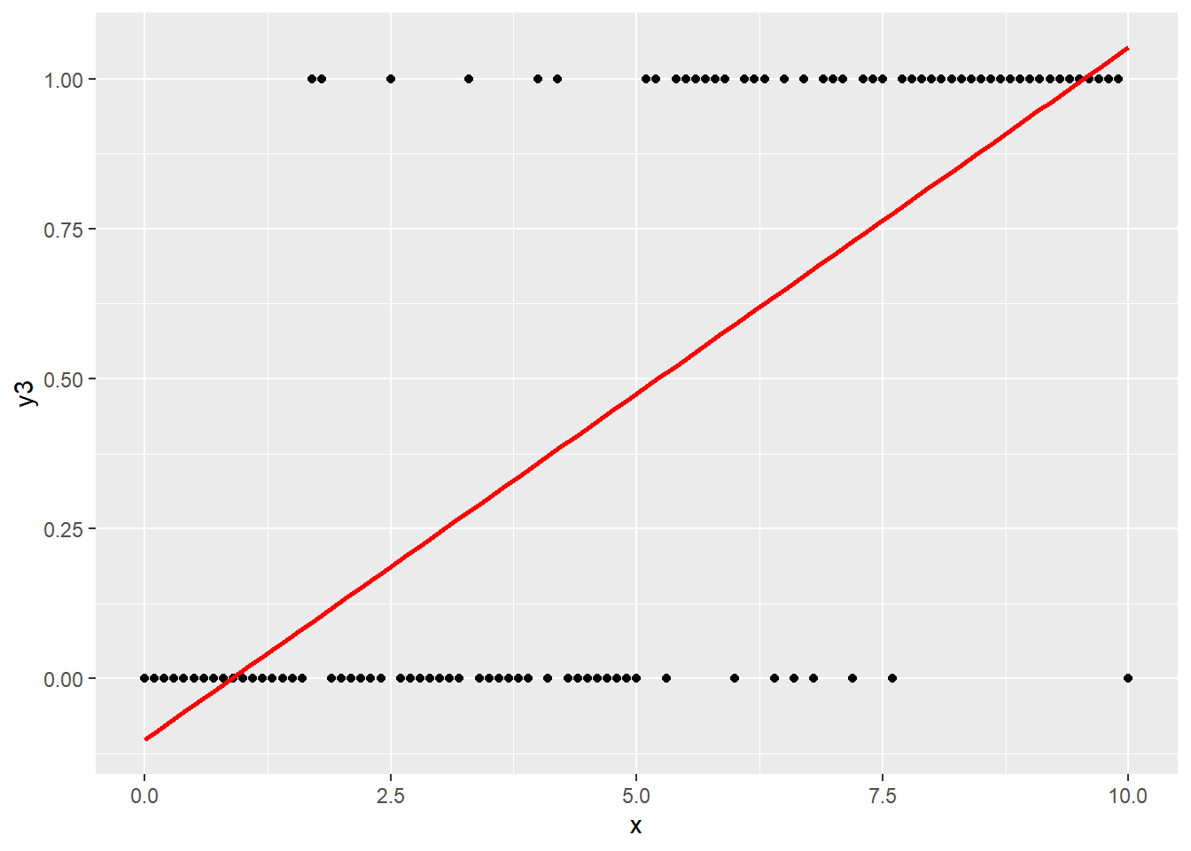 Because the data is more likely to be higher as
 x is larger, the best fit linear line has positive slope. However, it does not really capture the behavior of the data.
Instead of directly modeling the data using a linear model, let \(p\) be the probability that the data is 1, and \(1 - p\) be the probability that it is 0. Then \(p\) can be modeled using a logistic (logit for short) function.
If the probability of one outcome is \(p\), and the probability of another outcome is \(1 - p\), then the logit function is the logarithm of the odds of the first outcome to the second outcome. That is, \[ \operatorname{logit}(p) = \log\left(\frac{p}{1 - p}\right). \]
With this definition \(\operatorname{logit}(p)\) can be any positive or negative real number. The idea of logistic regression is to model \(\operatorname{logit}(p)\) using a linear function. That is, \[ \operatorname{logit}(p) = \log\left(\frac{p}{1 - p}\right) = \beta_0 + \beta_1 x_1 + \cdots + \beta_p x_p. \]
In R, the glm, or generalized linear models function, can be used to fit this model. The family = "binomial" option tells glm that the response variable is either 0 or 1.
Then add predictions.
Take a look:
## # A tibble: 6 × 2
##       x   pred
##   <dbl>  <dbl>
## 1   0   0.0243
## 2   0.1 0.0260
## 3   0.2 0.0278
## 4   0.3 0.0298
## 5   0.4 0.0319
## 6   0.5 0.0341
A bit hard to see from the first few points what the prediction looks like. Graphing this is a bit tricky, the y3 values should be used so that R treats it as a number rather than as a factor. The y-axis labels should just be 0 and 1. The scale_y_continuous can ensure that this happens.
ggplot(data = df3, aes(x)) +
  geom_point(aes(y = y3)) +
  geom_line(data = df4_pred,
            aes(x, pred),
            color = "red",
            lwd = 3) +
  scale_y_continuous('default', breaks = 0:1)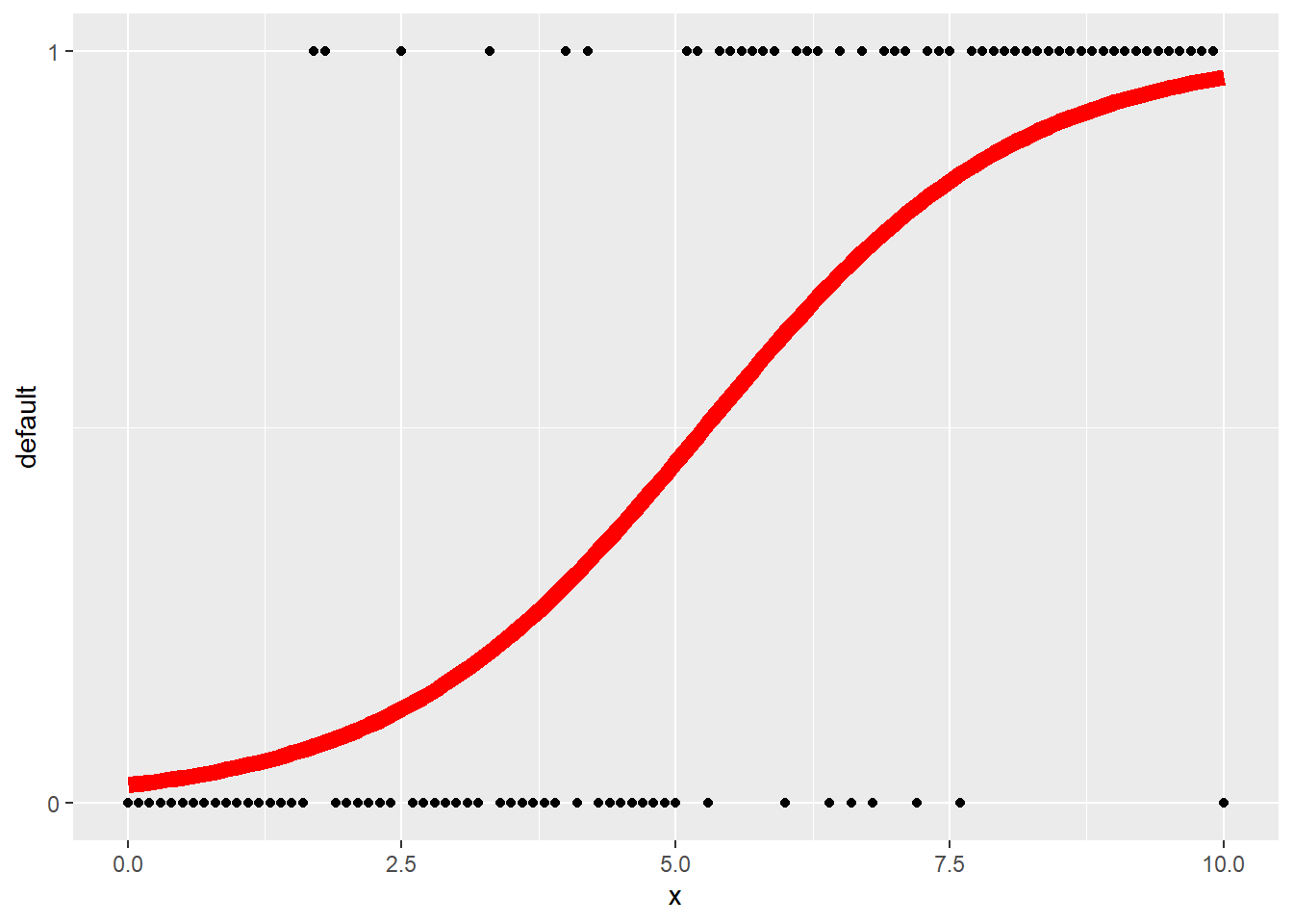
That S-shaped curve is the logistic curve, which gives this regression its name.
A simple prediction method is then: if \(p \geq 0.5\) predict 1, otherwise predict 0. Note that this is very close to what the decision tree would do for this data set. For this random data, it makes the cutoff greater than 5, without more data it will be unable to pinpoint the change point.
21.2.4 Boosting
Boosting tries to improve methods such as logistic regression by repeating them over multiple levels of prediction. We begin with some weak classifier that does not overfit. Logistic regression is often used for this.
At this point, if we just look at the predictions for our classifier on our training data set, we have made mistakes. So build a second classifier that gives more weight to the observations where we were mistaken. This gives us a second classifier.
We can repeat this process to obtain a family of classifiers. Now, just as in the random forests, we can run each of these classifiers to obtain a family of predictions. Then go with the prediction that is most popular among the family.
21.2.5 Support Vector Machines
A support vector machine classifies by trying to split the data into two groups using a hyperplane. In some cases, this is very easy, and the hyperplane can be used directly.
In other cases, the groups are separated by a curve. In order to deal with data like this, we need to develop a feature, a function of the predictors that gives a new predictor. Then we apply the hyperplane to this new feature.
A feature is a new predictor whose value is a function of other predictors.
21.2.6 Bayesian Classifiers/Bayesian Networks
Suppose that given which class an observation is in, the probability of certain predictor values appearing is known. Then Bayes Rule allows us to reverse the calculation and use predictor values to find the chance that a data point falls in a particular class.
These methods are in some sense the gold standard of classification. However, applying Bayes’ Rule to complex models is computationally very expensive.
The computations can be simplified by making assumptions about the model. The most basic assumption is that the predictors are conditionally independent given the class of the observation. That is, once we know which class we are in, all the predictors are independent of each other! Although this is a very powerful assumption, it can actually give models that are very useful for making predictions.
21.2.6.0.1 Neural Networks
A neural network tries to understand how the input and output variables of a model connect through a graph. In mathematics, a graph consists of nodes (also called vertices) that are connected by edges. Inputs to nodes become outputs to other nodes through the weights on the edges.
This process was inspired by biological neurons, which fire to other neurons when they are excited. Although mathematical neural networks are somewhat different from this process, the name has stuck, which is why they are called neural networks.
By using the data in observations, the weights on the edges are fine-tuned to make the final output of the graph equal to the input.
21.2.6.0.2 Deep Learning
Neural networks turned out to be difficult to use in complex situations. However, by first broadening the classifications to larger groups, a neural network works quite well. Then these broader classes can be refined. Do this three or four times, and we can get back to the original classes that we had in mind.
This is the basic idea behind deep learning. Use a nested set of neural networks (or other models) to slowly move from the input space to the output space. This idea has proved especially effective in areas such as computer vision, speech recognition, and natural language processing where the data naturally lends itself to large groups, then smaller more refined groups.
21.3 Unsupervised learning
In unsupervised learning, we are not given any labeled data. It is up to the algorithm to construct the classes that the observations fall into.
21.3.1 Clustering
An example of this type of learning is cluster analysis or more simply, clustering. Here the goal is to determine which observations in the sample space are close together to one another.
As with most models, there is no one right clustering. Instead, different clustering algorithms will achieve different results. In the end, the question is whether or not the clustering is useful for the purposes that the person analyzing the data is trying to achieve.
For example, suppose that each observation is a numerical \(n\)-tuple. Then a simple way to cluster is to calculate the distance between each pair of points. Setting a threshold value, connect any pairs of points whose distance is below that threshold. The number of clusters equals the number of points when the threshold is 0, and decreases as the threshold is raised.
Another type of clustering is based upon kernel density estimation. Here a normal density is placed on top of each point in the data set and then added up. For instance, suppose we have some \(x\) values drawn using a normal distribution centered at 3, and others drawn using a normal distribution centered at 8. This gives bimodal data. Then the kernel density plot might look as follows.
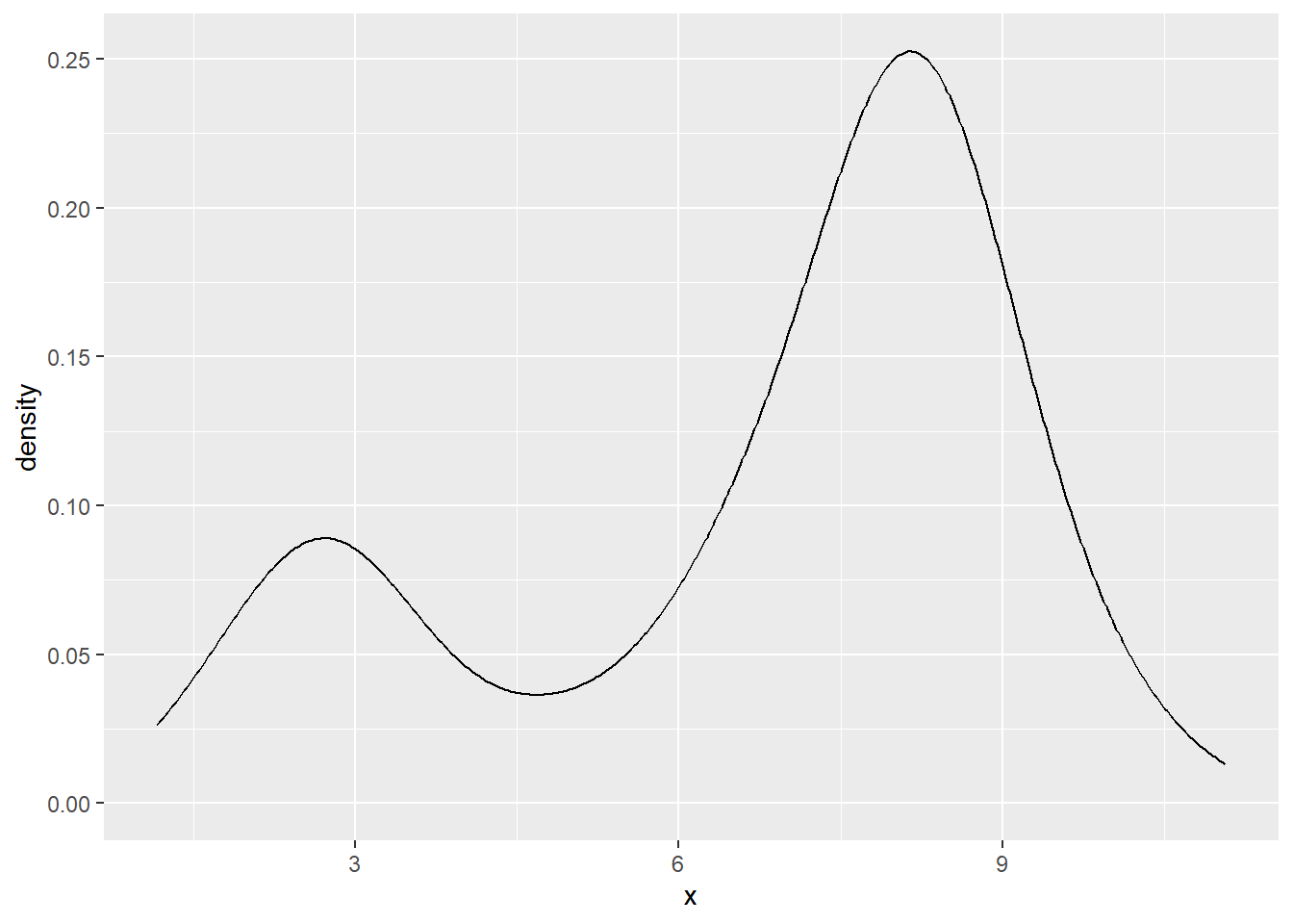
This kernel density plot has two local maxima, which separated the data points into two clusters. More generally this idea is known as density-based clustering.