18 Creating models
Summary
Models come from both base R and other packages.
- lm Creates a linear model.
The package modelr contains functions for evaluation of models.
data_grid Creates grid of unique prediction values.
add_predictions Calculates the predictions from the predictor variable values for a given model.
This chapter will use several functions and datasets from the modelr library.
18.1 The lm model in base R
Consider the dataset sim1 built into modelr.
## # A tibble: 30 × 2
##        x     y
##    <int> <dbl>
##  1     1  4.20
##  2     1  7.51
##  3     1  2.13
##  4     2  8.99
##  5     2 10.2
##  6     2 11.3
##  7     3  7.36
##  8     3 10.5
##  9     3 10.5
## 10     4 12.4
## # ℹ 20 more rows
The linear model that uses \(x\) to predict \(y\) is \(y = c_0 + c_1 x + \epsilon\). This model can be built in a more compact way using the lm function that is built into R. The function lm takes as its first input a formula form of the model. In this formula, the variable being predicted comes first, followed by a ~ symbol, followed by the predictor variables on the right.
For the simple model where x predicts y, the formula is then y ~ x. The second input to the model is the data itself. Therefore, to create the linear model, use
##
## Call:
## lm(formula = y ~ x, data = sim1)
##
## Coefficients:
## (Intercept)            x
##       4.221        2.052
The output displayed is the call to the model, together with the coefficients for the least squares estimates for the \(y\) intercept and the slope associated with \(x\). The model actually makes much more, which can be stored with a variable assignment.
It is actually pretty rare to have just one prediction variable. If the model includes \(n\) different predictor variables, the linear model can be expanded to \[ y = c_0 + c_1 x_1 + \cdots + c_n x_n + \epsilon. \]
Consider sim4, which holds variables x1, x2, rep, and y.
## # A tibble: 300 × 4
##       x1     x2   rep       y
##    <dbl>  <dbl> <int>   <dbl>
##  1    -1 -1         1  4.25
##  2    -1 -1         2  1.21
##  3    -1 -1         3  0.353
##  4    -1 -0.778     1 -0.0467
##  5    -1 -0.778     2  4.64
##  6    -1 -0.778     3  1.38
##  7    -1 -0.556     1  0.975
##  8    -1 -0.556     2  2.50
##  9    -1 -0.556     3  2.70
## 10    -1 -0.333     1  0.558
## # ℹ 290 more rows
If x1 and x2 are used to predict y, then the model becomes as follows.
A look at the model reveals the fitted coefficients.
##
## Call:
## lm(formula = y ~ x1 + x2, data = sim4)
##
## Coefficients:
## (Intercept)           x1           x2
##     0.03546      1.82167     -2.78252
Note that there is still an intercept, but now there is a coefficient (a slope) for each of x1 and x2. From this fit, the best prediction for \(y\) given \(x_1 = 2\) and \(x_2 = 3\) would be
\[
\hat y = 0.03546 + 1.82167(2) - 2.78252(3).
\]
18.1.0.1 Least squares ( \(L_2\) ) versus absolute value ( \(L_1\) )
The lm only fits using least squares, and cannot find the \(L_1\) distance. This is because there exists a polynomial time deterministic algorithm for calculating the values exactly for \(L_2\), but not for \(L_1\). In order to find the \(L_1\) fit, it is necessary to use optim. However, this function is not guaranteed to find the best solution (although it usually does on typical data). The optim function is slower, but applies to a wider variety of models.
18.2 Functions of the modelr package
In the work above, the linear model was implemented directly in R. Unfortunately, that does not always translate well to other models. The idea of the modelr package is to create a set of functions that work with all possible models.
Recall that by using the lm function, a linear model was created. Then functions in modelr can be called to make predictions using that model and to find the errors associated with the model using the actual data. The important thing is that these functions work no matter what the model is! That is, if instead of using lm, another type of model had been used, the same functions could still be called to get predictions and errors. This gives the user great flexibility in modeling the data.
In the last chapter, the predictions and residuals for a model were calculated directly. Here the add_predictions and add_residuals functions will be used to calculate these values for any model.
18.3 The add_predictions function
Given a particular model, the add_predictions function is a fast way of finding what the predicted value of a variable is given the values of predictor models used in the model.
For instance, recall that the sim1 data can be modeled using a linear model using the lm function. The resulting model was stored in the variable sim1_mod. Let’s take a look at this model.
##
## Call:
## lm(formula = y ~ x, data = sim1)
##
## Coefficients:
## (Intercept)            x
##       4.221        2.052
The main information that it shows is the function call used to create the model, and the coefficients of the best fit least squares line.
From this, it is possible to write a function that creates a prediction for y given x. However, the nice thing about using the add_predictions function instead is that it works regardless of what the model is. It saves the user from having to build these functions on their own.
The first parameter to add_predictions is a tibble/data frame that holds the values of x, and then the second is the model itself.
## # A tibble: 3 × 2
##       x  pred
##   <dbl> <dbl>
## 1   2.5  9.35
## 2   5.1 14.7
## 3   9.6 23.9
The values are stored in the variable pred. Plotting these predictions with the original data shows how these predictions look. Here the parameter data in the geom_point functions will be used to plot data from sim1 and from the predictions made above.
g <- ggplot() +
  geom_point(data = sim1, aes(x, y)) +
  geom_point(data = first_pred, aes(x, pred), color = "red", size = 3)
g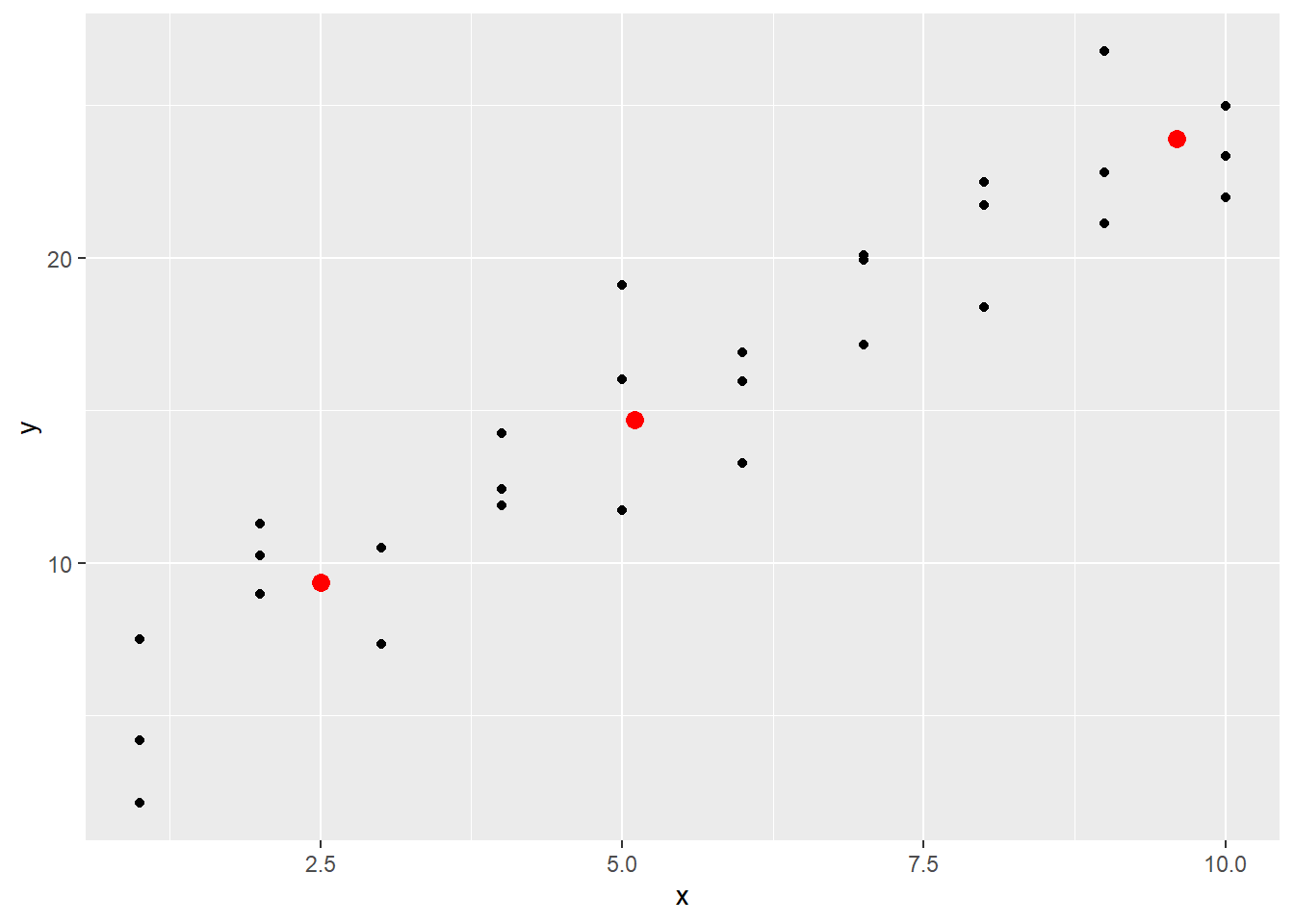
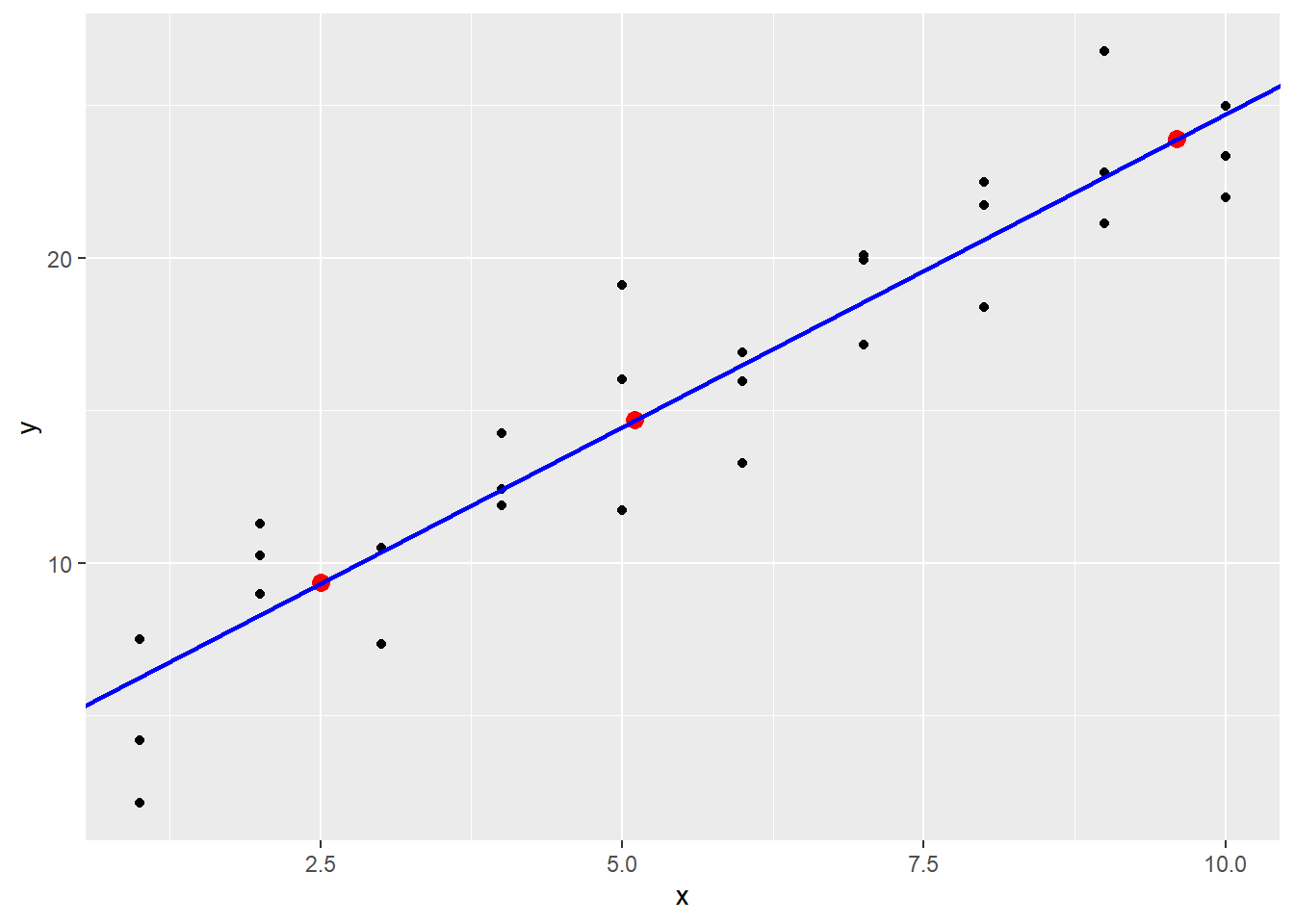
These lie on a line, and by using abline it becomes clear that these predictions are coming from the linear model stored in sim1_mod when the coefficients are added manually.
18.3.1 The data_grid function
In the above call to add_predictions, the x values were set up directly. Often, it is the case that the user wishes to have a prediction for each of the x values that appears in the data. That is where the data_grid function comes in.
This function takes a data set, and pulls out all possible values of the x variable. Applied to the sim1 dataset, it pulls out all the different x values in that dataset.
## # A tibble: 10 × 1
##        x
##    <int>
##  1     1
##  2     2
##  3     3
##  4     4
##  5     5
##  6     6
##  7     7
##  8     8
##  9     9
## 10    10
This data grid can then be used to obtain predictions where data already exists.
## # A tibble: 10 × 2
##        x  pred
##    <int> <dbl>
##  1     1  6.27
##  2     2  8.32
##  3     3 10.4
##  4     4 12.4
##  5     5 14.5
##  6     6 16.5
##  7     7 18.6
##  8     8 20.6
##  9     9 22.7
## 10    10 24.7
Visually, this looks as follows.
ggplot() +
  geom_point(data = sim1, aes(x, y)) +
  geom_point(data = grid_pred, aes(x, pred), color = "red", lwd = 3)
## Warning in geom_point(data = grid_pred, aes(x, pred), color = "red", lwd = 3):
## Ignoring unknown parameters: `linewidth`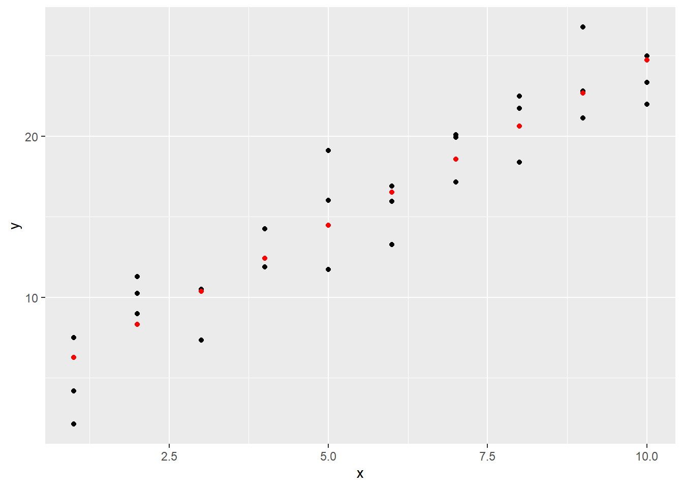
These predictions can also be visualized on a line.
ggplot() +
  geom_point(data = sim1, aes(x, y)) +
  geom_line(data = grid_pred, aes(x, pred), color = "red", lwd = 1)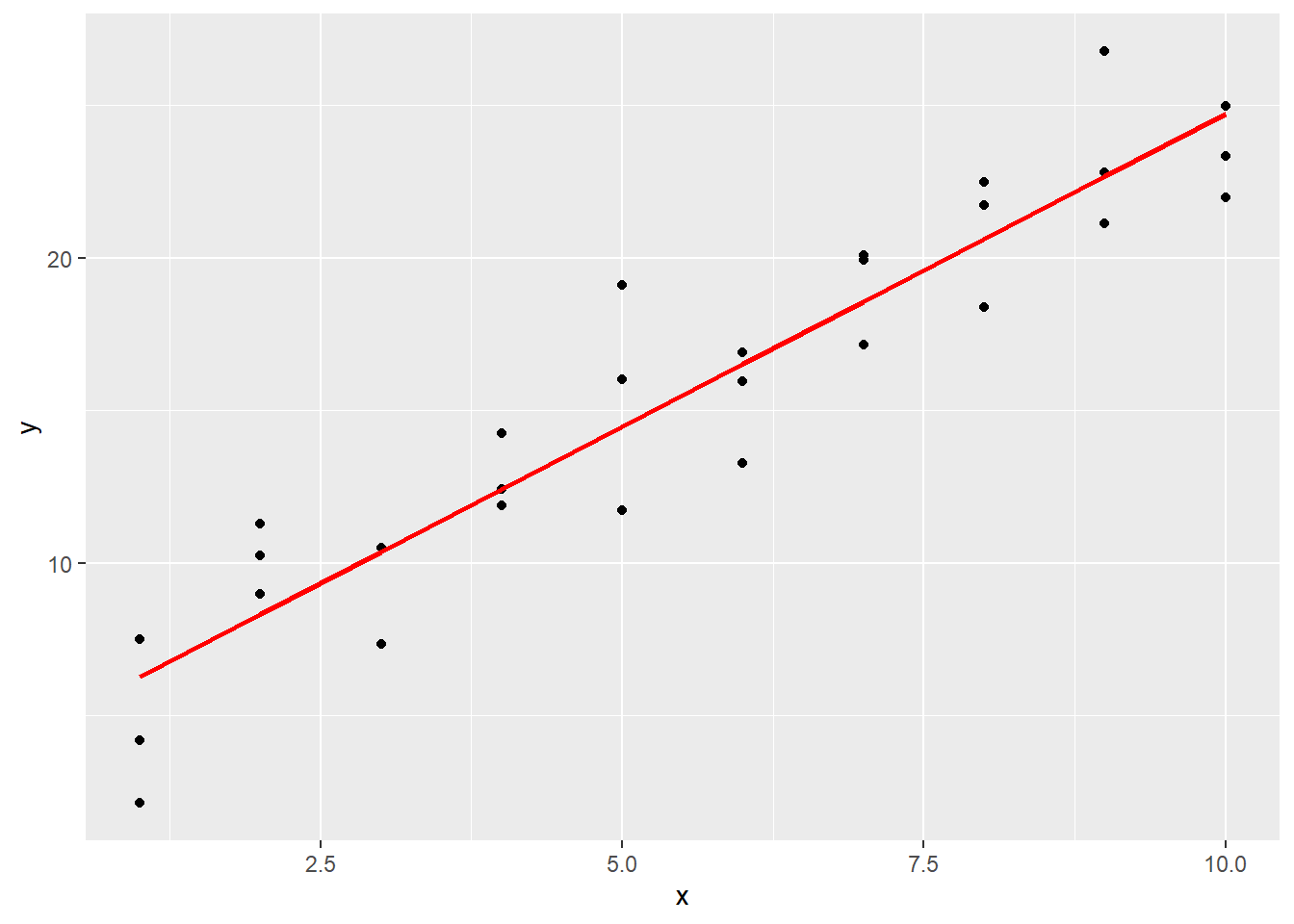
18.4 Models with more than one predictor variable
Earlier the data in sim4 was considered.
| x1 | x2 | rep | y |
|---|---|---|---|
| -1 | -1.0000000 | 1 | 4.2476777 |
| -1 | -1.0000000 | 2 | 1.2059970 |
| -1 | -1.0000000 | 3 | 0.3534777 |
| -1 | -0.7777778 | 1 | -0.0466581 |
| -1 | -0.7777778 | 2 | 4.6386899 |
| -1 | -0.7777778 | 3 | 1.3770954 |
The model sim4_mod was constructed with both x1 and x2 as predictor variables.
##
## Call:
## lm(formula = y ~ x1 + x2, data = sim4)
##
## Coefficients:
## (Intercept)           x1           x2
##     0.03546      1.82167     -2.78252
The add_predictions function handles this new model easily.
## # A tibble: 300 × 4
##       x1     x2   rep       y
##    <dbl>  <dbl> <int>   <dbl>
##  1    -1 -1         1  4.25
##  2    -1 -1         2  1.21
##  3    -1 -1         3  0.353
##  4    -1 -0.778     1 -0.0467
##  5    -1 -0.778     2  4.64
##  6    -1 -0.778     3  1.38
##  7    -1 -0.556     1  0.975
##  8    -1 -0.556     2  2.50
##  9    -1 -0.556     3  2.70
## 10    -1 -0.333     1  0.558
## # ℹ 290 more rows
#sim4 |>
# data_grid(x1, x2) |>
# add_predictions(sim4_mod) |>
# left_join(sim4 |> select(x1, x2, y), by = c("x1", "x2")) |>
# head() |> kable() |> kable_styling()18.4.1 Handling relationships between predictor variables
In the previous example, the predictor variables x1 and x2 were independently measured. However, it is possible for one predictor variable to be a function of another. For instance, \(x\) and \(x^2\) might be a predictor for \(y\).
To deal with this, if x is a factor, then make x_square a factor using mutate, and use in the model as well.
To see this in action, first generate some data from the model
\[
y = 0.5 - 2 x + 0.2 x^2 + \epsilon.
\]
The original prediction variable was x. The mutate can be used to build the new variable x_square with values equal to the squares of the x values, along with some randomly generated \(\epsilon\) values created using the rnorm function.
set.seed(123456) # makes the random numbers come out the same way each time
x <- 1:10
sim5 <- tibble(x = c(x, x)) |>
  mutate(x_square = x^2) |>
  mutate(y = 0.5 - 2 * x + 0.2 * x_square +
             1.1 * rnorm(length(x)))

sim5 |>
  ggplot() +
    geom_point(aes(x, y))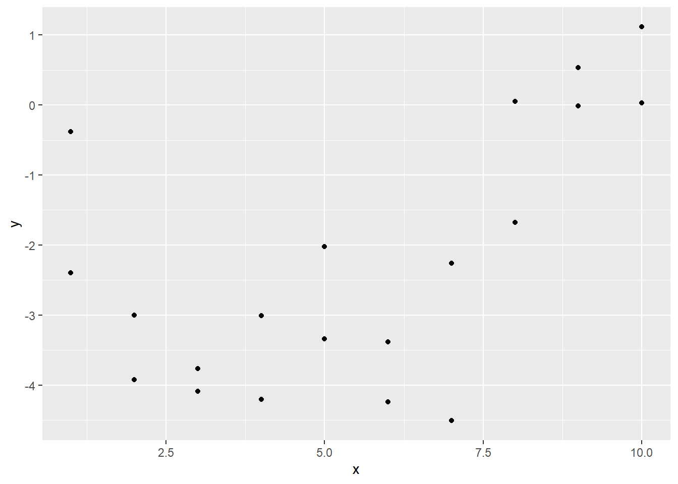
Now use lm to fit this model to the data:
## (Intercept)           x    x_square
##  -0.8217856  -1.3251656   0.1528941
In this model, both x and x_square are predictors, since they are both multiplied by coefficients and added together.
With this model there is a bit of caution necessary. The data_grid function does not recognize that x_square is a function of x. Therefore, you can use it to pull out the x variable, but then the x_square variable must be created separately.
grid5_pred <-
  sim5 |>
    data_grid(x) |>
    mutate(x_square = x^2) |>
    add_predictions(sim5_mod)
grid5_pred
## # A tibble: 10 × 3
## x x_square pred
## <int> <dbl> <dbl>
## 1 1 1 -1.99
## 2 2 4 -2.86
## 3 3 9 -3.42
## 4 4 16 -3.68
## 5 5 25 -3.63
## 6 6 36 -3.27
## 7 7 49 -2.61
## 8 8 64 -1.64
## 9 9 81 -0.364
## 10 10 100 1.22Now plot the original data together with the predictions.
ggplot(sim5, aes(x)) +
  geom_point(aes(y = y)) +
  geom_line(data = grid5_pred,
            aes(x = x, y = pred),
            color = "red", size = 1)
## Warning: Using `size` aesthetic for lines was deprecated in ggplot2
## 3.4.0.
## ℹ Please use `linewidth` instead.
## This warning is displayed once every 8 hours.
## Call `lifecycle::last_lifecycle_warnings()` to see where
## this warning was generated.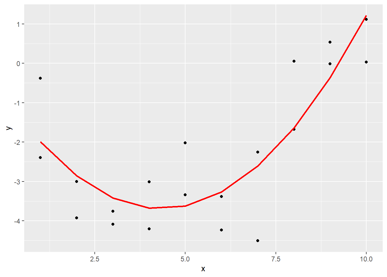
Note that this is still a linear model, even though the prediction line is a quadratic function. The linear in linear model refers to the fact that each predictor (\(x\) and \(x^2\)) is multiplied by a constant and added together. Other functions of \(x\) like \(\exp(x)\) and \(\sin(x)\) could have also been part of the prediction! So linear models include an incredibly wide range of models, just by themselves!