14 Factors
Summary
The values that categorical variables can take on are called levels, and there are several functions designed to assist in modifying the order and name of levels. Some of these are in base R, while others are part of the tidyverse package forcats.
factor gives the factor values for a variable and the permissible levels.
unique finds the levels for a variable by looking at the unique values that the variable takes on.
fct_infreq takes in a dataset and turns it into a factor whose levels are in the order of the frequency of values in the dataset.
fct_reorder reorders the levels of a single factor.
fct_reorder2 reorders the levels of a single factor by considering values of a second factor as well.
fct_relevel pushes a level to the end of the factor order.
fct_recode can be used to rename all the levels of a factor.
fct_collapse can combine different levels into one level.
fct_lump automatically combines the uncommon levels for a variable.
14.1 What is a factor?
Recall that in tidy data, each column corresponds to a variable that is also known as a factor. That means a factor is something that can be measured, and the values that each measurement can take on are called levels. In categorical data, the data only takes on a finite set of values. For instance, month, blood type, and religion are typical examples of categorical variables. A numerical measurement like height or income would typically not be considered categorical.
In tidy data, a variable is also called a factor.
The values that a factor can take on are called levels.
14.2 Ordering levels in factors
One of the benefits of treating variables as factors is when it comes to ordering levels. Consider the following set of data recording months in which four events occurred.
There are several problems that can arise with this type of data. First, it is easy to make a typo that moves us outside of the set of months.
Second, if the data is sorted, the order of the sort will be alphabetical. But months have a particular order in which they should be sorted.
## [1] "Apr" "Dec" "Duc" "Jan"To fix the first problem, the permissible level values and their proper order could be assigned as part of the factor.
Note that in months, the levels are in proper month order.
The factor function can be used to tell R exactly what the levels are for a particular variable.
## [1] Dec Dec Apr Jan
## Levels: Jan Apr Dec
Looking at y1 reveals that there are two types of information contained within: the actual data and the levels for the factor.
Sorting now works because it respects the level order.
## [1] Jan Apr Dec Dec
## Levels: Jan Apr Dec
If (as in factor2) a data value is not a level, it will return an NA.
## [1] <NA> Dec  Apr  Jan
## Levels: Jan Apr Dec
It is not always possible to know the level order ahead of time. For many datasets, the usual order is the first appearance of the level in the data itself. The unique function can be used to pull out the first appearance of the value within the data.
## [1] "Dec" "Dec" "Apr" "Jan"## [1] "Dec" "Apr" "Jan"## [1] Dec Dec Apr Jan
## Levels: Dec Apr Jan14.3 Package forcats
The tidyverse package for dealing with factors is called forcats, which is an acronym for categorical data sets. An acronym is an abbreviation formed from a subset of letters in a phrase that is pronounced as a word. Often acronyms are formed from the initial letters of a phrase. For instance, NOAA is an acronym for the National Oceanic and Atmospheric Administration, ICSC stands for the International Climate Science Coalition, and APAN stands for the Asia Pacific Adaption Network.
14.3.1 fct_infreq
One such function from this package is fct_infreq. This is similar to factor in that it takes a dataset and creates a factor, but here the levels are ordered first by the number of times a value appears, and then alphabetically.
## [1] red   red   green blue
## Levels: red blue green
14.3.2 The General Social Survey
The National Opinion Research Centers (NORC) conducts a poll called the General Social Survey (http://gss.norc.org/) which has for many years asked the US population about marriage, age, race, income, religion, and other factors.
The forcats package contains a variable gss_cat that is a small sample of the data set from the year 2000.
## # A tibble: 21,483 × 9
##     year marital         age race  rincome partyid relig denom
##    <int> <fct>         <int> <fct> <fct>   <fct>   <fct> <fct>
##  1  2000 Never married    26 White $8000 … Ind,ne… Prot… Sout…
##  2  2000 Divorced         48 White $8000 … Not st… Prot… Bapt…
##  3  2000 Widowed          67 White Not ap… Indepe… Prot… No d…
##  4  2000 Never married    39 White Not ap… Ind,ne… Orth… Not …
##  5  2000 Divorced         25 White Not ap… Not st… None  Not …
##  6  2000 Married          25 White $20000… Strong… Prot… Sout…
##  7  2000 Never married    36 White $25000… Not st… Chri… Not …
##  8  2000 Divorced         44 White $7000 … Ind,ne… Prot… Luth…
##  9  2000 Married          44 White $25000… Not st… Prot… Other
## 10  2000 Married          47 White $25000… Strong… Prot… Sout…
## # ℹ 21,473 more rows
## # ℹ 1 more variable: tvhours <int>
This is a tibble, so we can use our panoply of commands to learn more about it.
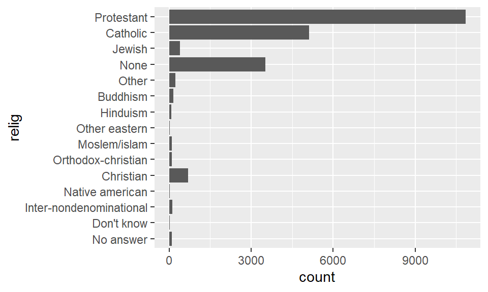
Everything on the left hand side is a level for the factor relig. Suppose we want to learn about the average age and average number of hours spent watching TV per day across religions.
relig_sum <- gss_cat |>
  group_by(relig) |>
  summarize(
    age = mean(age, na.rm = TRUE),
    tvhours = mean(tvhours, na.rm = TRUE),
    n = n()
  )

relig_sum |>
  ggplot() +
  geom_bar(aes(relig, tvhours), stat = 'identity') +
  coord_flip()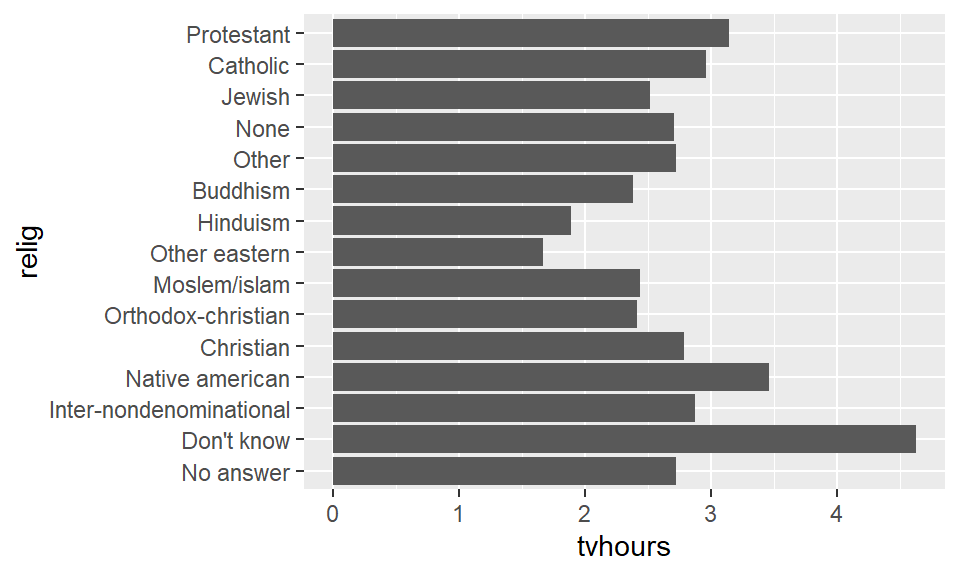
14.4 Ordering the levels for visualizations
In this case the order of the levels is not exactly helpful. So we want to reorder the factor levels based on the TV hours viewed. The function fct_reorder accomplishes exactly this task. For instance:
relig_sum |>
  ggplot() +
    geom_bar(aes(fct_reorder(relig, tvhours), tvhours),
             stat = 'identity') +
  coord_flip()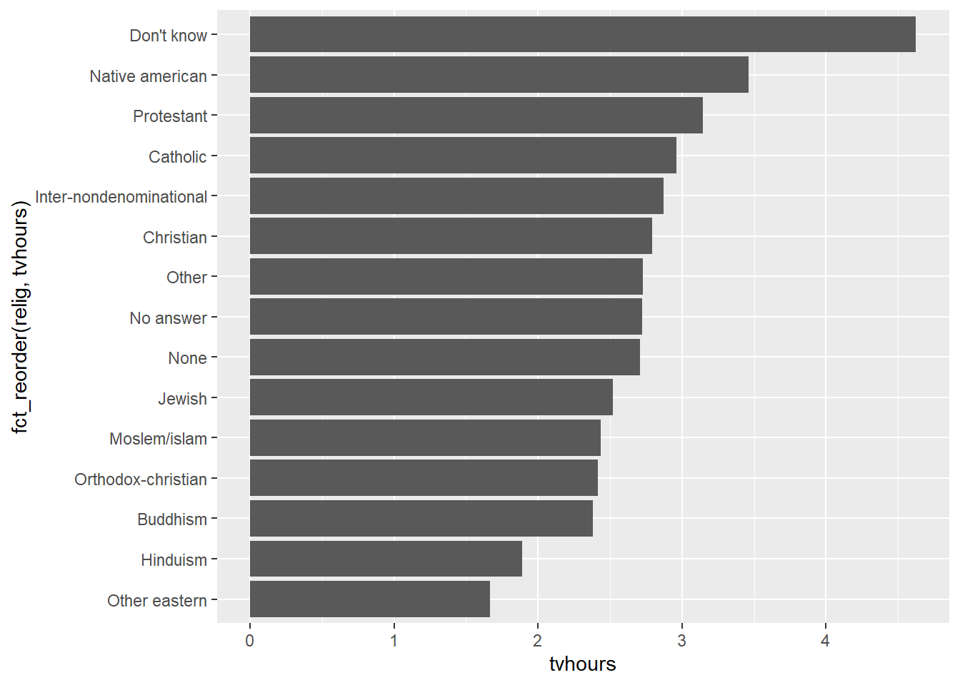
It is much easier with this level ordering to see how much TV viewing hours in 2000 changed with religion.
The same reordering could have been accomplished by directly mutating the relig factor as well.
relig_sum |>
  mutate(relig_bytv = fct_reorder(relig, tvhours)) |>
  ggplot() +
    geom_bar(aes(relig_bytv, tvhours), stat = 'identity') +
    coord_flip()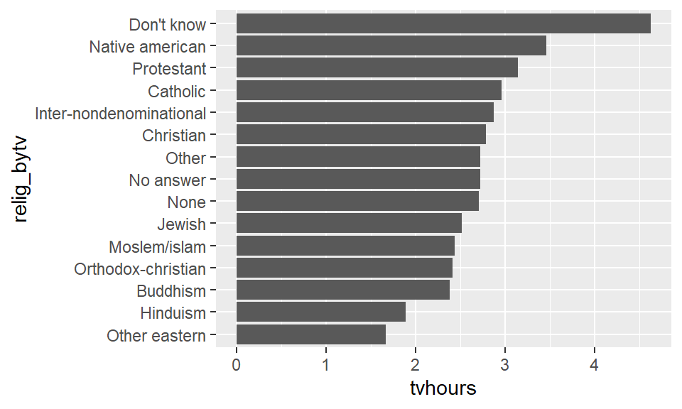
Note that a couple of these answers for religion are not like the others. For instance, we have "Don't know", "Other", "None", and "No answer". These of course are not religions in and of themselves. We can move a level to the front of the line using the fct_relevel command.
relig_sum |>
  mutate(relig_bytv = fct_reorder(relig, tvhours)) |>
  ggplot() +
    geom_bar(aes(fct_relevel(relig_bytv, "No answer"),
                 tvhours), stat = 'identity') +
    coord_flip()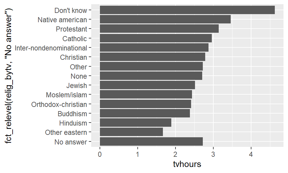
The function fct_reorder2 can be useful when we are doing line plots in color. This function lines up the lines so that they are ordered by the last value. This makes the lines match up correctly with the labels in the legend, which makes the legend much easier to read.
by_age <- gss_cat |>
  filter(!is.na(age)) |>
  count(age, marital) |>
  group_by(age) |>
  mutate(prop = n / sum(n))

ggplot(by_age, aes(age, prop, color = marital)) +
  geom_line(na.rm = TRUE)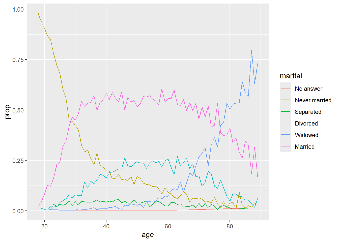
ggplot(by_age, aes(age, prop,
                   color = fct_reorder2(marital, age, prop))) +
  geom_line() +
  labs(color = "marital")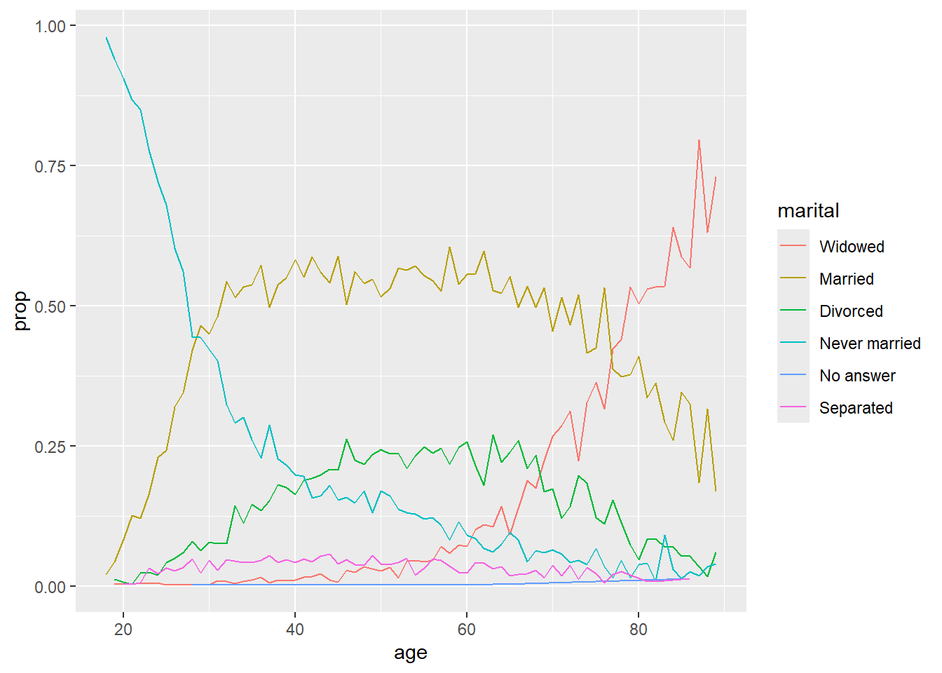
14.5 Changing the levels
It might be the case that we wish to change the actual names of the levels for clarity or for a particular graphic. The fct_recode accomplishes this task. Consider:
## # A tibble: 10 × 2
##    partyid                n
##    <fct>              <int>
##  1 No answer            154
##  2 Don't know             1
##  3 Other party          393
##  4 Strong republican   2314
##  5 Not str republican  3032
##  6 Ind,near rep        1791
##  7 Independent         4119
##  8 Ind,near dem        2499
##  9 Not str democrat    3690
## 10 Strong democrat     3490
There are three parties hiding in there: Republican, Independent, and Democratic. However, the adjectives come before Republican and Democrat, and after Independent. Moreover, each should be capitalized. We can fix these with a recode.
gss_cat |>
  mutate(partyid = fct_recode(partyid,
    "Republican, strong"    = "Strong republican",
    "Republican, weak"      = "Not str republican",
    "Independent, near rep" = "Ind,near rep",
    "Independent, near dem" = "Ind,near dem",
    "Democrat, weak"        = "Not str democrat",
    "Democrat, strong"      = "Strong democrat"
  )) |>
  count(partyid)
## # A tibble: 10 × 2
## partyid n
## <fct> <int>
## 1 No answer 154
## 2 Don't know 1
## 3 Other party 393
## 4 Republican, strong 2314
## 5 Republican, weak 3032
## 6 Independent, near rep 1791
## 7 Independent 4119
## 8 Independent, near dem 2499
## 9 Democrat, weak 3690
## 10 Democrat, strong 3490Because we did not mention some of the levels (for instance, “No answer”), that level stayed exactly the same as before. We can also use fct_recode to combine several labels into 1.
gss_cat |>
  mutate(partyid = fct_recode(partyid,
    "Republican"    = "Strong republican",
    "Republican"      = "Not str republican",
    "Independent" = "Ind,near rep",
    "Independent" = "Ind,near dem",
    "Democrat"        = "Not str democrat",
    "Democrat"      = "Strong democrat",
    "Other"                 = "No answer",
    "Other"                 = "Don't know",
    "Other"                 = "Other party"
  )) |>
  count(partyid)
## # A tibble: 4 × 2
## partyid n
## <fct> <int>
## 1 Other 548
## 2 Republican 5346
## 3 Independent 8409
## 4 Democrat 7180If you wish to collapse multiple levels, a function that makes code easier to read is fct_collapse. Here we can give each new level a vector of old levels to collapse down to.
gss_cat |>
  mutate(partyid = fct_collapse(partyid,
    other = c("No answer", "Don't know", "Other party"),
    rep = c("Strong republican", "Not str republican"),
    ind = c("Ind,near rep", "Independent", "Ind,near dem"),
    dem = c("Not str democrat", "Strong democrat")
  )) |>
  count(partyid)
## # A tibble: 4 × 2
## partyid n
## <fct> <int>
## 1 other 548
## 2 rep 5346
## 3 ind 8409
## 4 dem 7180If you don’t want to deal with anything but the labels with the largest counts, the fct_lump command does this automatically.
## # A tibble: 2 × 2
##   relig          n
##   <fct>      <int>
## 1 Protestant 10846
## 2 Other      10637
The most important parameter here is n, which says how many groups we wish to end up with.
gss_cat |>
  mutate(relig = fct_lump(relig, n = 10)) |>
  count(relig, sort = TRUE) |>
  print(n = Inf)  # show all rows of the tibble.
## # A tibble: 10 × 2
## relig n
## <fct> <int>
## 1 Protestant 10846
## 2 Catholic 5124
## 3 None 3523
## 4 Christian 689
## 5 Other 458
## 6 Jewish 388
## 7 Buddhism 147
## 8 Inter-nondenominational 109
## 9 Moslem/islam 104
## 10 Orthodox-christian 95Questions
Consider the data:
Create a new dataset with the levels into the proper month order.
Create a bar plot of the data and place this graphical object.
Consider the variable blood.
blood <- c("B", "A", "A", "A", "A", "AB", "O", "B", "A", "B", "A", "A", "B", "A", "AB", "AB", "O", "A", "B", "A")This contains blood types that are either type "A", "B", "AB", or "O". Turn this into a factor with levels in that order.
Continuing the last problem, suppose now there are types "A-" (read as A negative), "A+" (read as A positive), "B-", "B+", "AB-", "AB+", "O-", and "O+".
blood_rh <- c("B+", "A+", "A+", "A-", "A-", "AB-", "O-", "B-", "A-", "B+", "A+", "A-", "B+", "A-", "AB+", "AB-", "O+", "A-", "B+", "A+")Write code to collapse the dataset blood_rh down to the four blood types from the previous problem.
Consider the gss_cat variable from the forcats.
The count can be used to tell how many observations there are for each age and relig value.
## # A tibble: 735 × 3
##    relig       age     n
##    <fct>     <int> <int>
##  1 No answer    19     1
##  2 No answer    22     1
##  3 No answer    24     1
##  4 No answer    25     1
##  5 No answer    26     3
##  6 No answer    28     1
##  7 No answer    29     2
##  8 No answer    30     2
##  9 No answer    32     3
## 10 No answer    34     2
## # ℹ 725 more rows
Using this data, create a graph showing how the proportion of religious affiliation varies with age. Make your graph as readable as possible by properly ordering the levels in the legend.
Consider the data set ad_treatment.xlsx that can be found at https://s3.us-west-1.amazonaws.com/markhuber-datascience-resources.org/Data_sets/ad_treatment.xlsx. Read this in using download.file and the function read_xlsx from the realxl library.
What are the factors of this dataset?
Write code to report the levels of the factor
drug_treatment.